Graph #2: best fit Lines for the increasing part of the data:
- Best Fit #1polynomial that is represented by the gray portion graph #2 is a polynomial function to the power 7 with equation:
Y1a= (-1.762×10-11 ×7) + (3.116×10-5 ×6) + (- 0.00214×5) + (0.0718×4) + (-1.229×3) + (10.44×2) + (- 30.774×) + (440.834)
- Best Fit #2 exponential that is represented by the black portion on graph #2 is an exponential function with equation:
Y1b = 338.129 e 0.030 ×
Graph #3: Best fit lines for the decreasing part of the Data
- Best Fit #1 polynomial represented by the black portion on graph #3 is a polynomial function of power 7 with equation:
Y2a= (-7.298×10-11×7) + (1.183×10-7×6) + (-5.665×10-5×5) + (0.013×4) + (-1.624×3) + (114.783×2) + (- 4316.0849×) + (69060.761)
- Best Fit #2 exponential represented by the gray portion on graph #3 is an exponential function with equation:
Y2b = 3163.562 e -0.0116x
And so as we can see from the graphs above, the polynomial function are more suitable to be used as best fit functions from the exponential functions.
From this we can say that the function (polynomial) for the increasing part of the original data for the flow rate of the Nolichucky River in Tennesse:
Y1= (-1.762×10-11 ×7) + (3.116×10-5 ×6) + (- 0.00214×5) + (0.0718×4) + (-1.229×3) + (10.44×2) + (- 30.774×) + (440.834)
While the function (polynomial) for the decreasing part is:
Y2= (-7.298×10-11×7) + (1.183×10-7×6) + (-5.665×10-5×5) + (0.013×4) + (-1.624×3) + (114.783×2) + (- 4316.0849×) + (69060.761)
Graph #3: The lines of best fit for all of the original data (the decreasing and the increasing part):
And from graph #3 above we can see that the function starts increasing from 0 hours till it reaches 54 hours and that is represented by the black part of the graph, but as we can see the graph starts decreasing at the beginning between 0 and 6 hours, then it starts increasing till it reaches 54 hour.
Also as we can see the function start decreasing after it reaches 54 hour till it reaches 144 hours, and this is represented by the gray part of the graph.
And from the above we can see that the river had its greatest rate of flow at 54 hour and that is at 6:00 o'clock on the 29th of October 2002, and in order to show this in a mathematical way we must derivate both equations and find their maximum point, since the derivative of a function show the rate of change of that function.
Derivative of Y1 (Y1′) = (-1.233×10-6×6) + (1.870×10-4×5) + (- 0.107×4) + (0.287×3) + (-3.687×2) + (20.880×) + (-30.774)
Derivative of Y2 (Y2′) = (-5.109×10-11×6) + (7.098×10-7×5) + (-2.832×10-4×4) + (0.052×3) + (-4.872×2) + (229.566×) + (-4316.0849)
And according to the original data we can see that at the 54 hours the rate of flow was 1920 cfs-1. And to check for the accuracy of our equations we substitute 54 in the place of × in one of the equations:
Y1 = (-1.762×10⁻¹¹ (54)7) + (3.116×10⁻⁵ (54)6) + (-0.00214(54)5) + (0.0718(54)4) + (-1.229(54)3) + (10.44(54)2) + (-30.774(54)) + (440.834)
Y1= 1921.429cfs-1
And from this we can see that our experimental value is very close to the actual value of flow, which makes our equation accurate.
And such increase and then decrease in the rate of flow of water could be formed by stormy weather, since the increase in the flow of wind in that area will increase the rate of flow, and an decrease in the flow of wind in that area will decrease the flow of water in the river.
The amount of water flowing past the measuring station between 00:00 on 28th of October 2002 and 00:00 on 29th of October 2002 and that is between 24 hours and 48 hours can be known using a definite integration:
And the result of this integration will be found using a graphic calculator which will give = 23694.477 cubic feet.
And to find when the flow rate was 1000 cfs-1, we must know that the flow rate was twice 1000 cfs-1, and one is on the increasing part of the function and the other is on the decreasing part of the function. And in order to find the two values we must put 1000 cfs-1 equal to both equations:
1000 = (-1.762×10⁻¹¹ (54)7) + (3.116×10⁻⁵ (54)6) + (-0.00214(54)5) + (0.0718(54)4) + (-1.229(54)3) + (10.44(54)2) + (-30.774(54)) + (440.834)
Therefore,
x= 38.611 hours (14:36 o'clock on the 28th of October)
Y2= 1000 = (-7.298×10-11×7) + (1.183×10-7×6) + (-5.665×10-5×5) + (0.013×4) + (-1.624×3) + (114.783×2) + (- 4316.0849×) + (69060.761)
Therefore,
× = 94.242 hours (22:15 o'clock on the 30th of October)
we can use the graphs of the derivative functions in order to know at which day did the amount of flowing water increase and by checking if they are above or below the x-axis to find if the function is decreasing or increasing, and if the graph of the derivative of the function is above the time - axis (x – axis) then the amount of flowing water is increasing.
Graph #4: Graph of the derivatives of the two functions:
And as we can see from graph #4 the amount of flowing water was increasing in the time periods from 02:00 of 27th of October until 06:00 of 29th of October and from 23:00 of 1st of November until 00:00 of 2nd of November. And at those times the dams of the river where opened, which explains the increase in the flow of water.
And in order to find the average values for the flow of water, we can use the Mean Value Theorem for Y1 and Y2 , and then we add the two values and divide them by 2.
= 858.83 cfs -1
=1047.39 cfs -1
Therefore,
cfs-1
And again we have two time periods at which the flow rate was equal to this value, and we can find them by putting 953.11 cfs-1 equal to Y1 and Y2
Y1 = 953.11 = (-1.762×10-11 ×7) + (3.116×10-5 ×6) + (- 0.00214×5) + (0.0718×4) + (-1.229×3) + (10.44×2) + (- 30.774×) + (440.834)
x= 36.1 hours (12:10 on 28th of October)
Y2 = 953.11= (-7.298×10-11×7) + (1.183×10-7×6) + (-5.665×10-5×5) + (0.013×4) + (-1.624×3) + (114.783×2) + (- 4316.0849×) + (69060.761)
x= 96.35 hours (01:20 on 31st of October)