Number of units produced 35,000 40,000 45,000
Number of units sold 35,000 40,000 45,000
Unit Selling price $ 30 $ 30 $ 30
- Full absorption costing method
Sales $1,050,000 $1,200,000 $1,350,000
Less: Cost of goods sold 840,000 960,000 1,080,000
Gross profit $ 210,000 $ 240,000 $ 270,000
Selling and administration expenses 45,000 50,000 48,000
Net income $ 165,000 $ 190,000 $ 222,000
- Variable costing method
Sales $ 1,050,000 $ 1,200,000 $ 1,350,000
Less: Cost of goods sold 665,000 760,000 855,000
Gross profit $ 385,000 $ 440,000 $ 495,000
Fixed manufacturing overheads 200,000 200,000 200,000
Selling and administration expenses 45,000 50,000 48,000
Net income $ 140,000 $ 190,000 $ 247,000
Reconciliation:
Net income per (a) $ 165,000 $ 190,000 $ 222,000
(Under)/Over absorption
Of manufacturing fixed overheads (25,000) - 25,000
Net income per (b) $ 140,000 $ 190,000 $ 247,000
Situation 2
Month 1 Month 2 Month 3
Number of units produced 35,000 40,000 45,000
Number of units sold 35,000 35,000 35,000
(a) Full absorption costing method
Sales $1,050,000 $1,050,000 $1,050,000
Less: Cost of goods sold 840,000 840,000 840,000
Gross profit $ 210,000 $ 210,000 $ 210,000
Selling and administration expenses 45,000 50,000 48,000
Net income $ 165,000 $ 160,000 $ 162,000
(b) Variable costing method
Sales $ 1,050,000 $1,050,000 $1,050,000
Less: Cost of goods sold 665,000 665,000 665,000
Gross profit $ 385,000 $ 385,000 $ 385,000
Fixed manufacturing overheads 200,000 200,000 200,000
Selling and administration expenses 45,000 50,000 48,000
Net income $ 140,000 $ 135,000 $ 137,000
Reconciliation:
Net income per (a) $ 165,000 $ 160,000 $ 162,000
(Under)/ Over absorption
Of manufacturing fixed overheads (25,000) - 25,000
Inventory change - (25,000) (50,000)
Net income per (b) $ 140,000 $ 135,000 $ 137,000
Situation 3
Month 1 Month 2 Month 3
Number of units produced 45,000 45,000 45,000
Number of units sold 35,000 40,000 45,000
(a ) Full absorption costing method
Sales $ 1,050,000 $1,200,000 $1,350,000
Less: Cost of goods sold 840,000 960,000 1,080,000
Gross profit $ 210,000 $ 240,000 $ 270,000
Selling and administration expenses 45,000 50,000 48,000
Net income $ 165,000 $ 190,000 $ 222,000
- Variable costing method
Sales $ 1,050,000 $1,200,000 $1,350,000
Less: Cost of goods sold 665,000 760,000 855,000
Gross profit $ 385,000 $ 440,000 $ 495,000
Fixed manufacturing overheads 200,000 200,000 200,000
Selling and administrative expenses 45,000 50,000 48,000
Net income $ 140,000 $ 190,000 $ 247,000
Reconciliation:
Net income per (a) $ 165,000 $ 190,000 $ 222,000
(Under)/Over absorption
of manufacturing overheads 25,000 25,000 25,000
Inventory change (50,000) (25,000) -
Net income per (b) $ 140,000 $ 190,000 $ 247,000
Management issues and impact on organizational behaviour
Although variable costing method of inventory valuation is not acceptable in financial and tax accounting, it has benefits when used appropriately in internal reporting and performance measurement. During slack periods, factory management tends to build inventory, in order to absorb manufacturing overheads when full absorption costing method is used. Under full absorption costing method, the more the factory produces( irrespective of whether the output can be sold or not), the more it absorbs the manufacturing fixed overheads. Therefore there is potential risk if the factory is treated as a profit center and full absorption costing method is used. The risk becomes even greater, when there are different products and specifications for different customers. If the factory produces without a customer order, customer specific products may end up becoming slow moving or even obsolete, if factory output is not well managed.
On the other hand, if inventory is valued at variable cost, product costs would not represent its true cost.If such product cost information is made available to sales personnel, there is likelihood that salesmen may offer lower prices in order to book more orders. Another perspective of treating manufacturing fixed overheads is that these are costs that would be incurred irrespective of whether the factory operates at full capacity or not. If this being the case, should the company sell at below the total cost but above the direct or variable costs when it comes under price pressure so that the company can fully utilize its factory capacity.
In the final analysis, management should take all possible situations into account in determining the course of action. More importantly, management decisions will need to be constantly reviewed and changes as required, based on internal as well as factors will have to be made. Responding to the external environment is critical to the success of the business. The choice between the two costing methods in pricing decisions and in managing the business and in directing the organizational organizational behaviour can contribute to the profitability of the business.
Inventory Management
A key decision in manufacturing , retail, and some service industry firms is how much inventory to keep on hand. Once inventory levels are established, they become an important input to the budgeting system. Inventory decisions involve a delicate balance between three classes of costs: ordering costs, holding costs, and shortage costs
Economic Order Quantity
SuperSports Inc., has expanded its product line into winter sports equipment. The company’s newest product is a fiberglass snowboard. One of the raw materials is a special resin to bind the fiberglass in the molding phase of production. The production manager, Tony Smith, uses an economic order quantity(EOQ) decision model to determine the size and frequency with which resin is ordered. An economic order quantity(EOQ) is the order size that minimizes inventory ordering and holding costs. The EOQ model is a mathematical tool for determining the order quantity that that minimizes the costs of ordering and holding inventory.
Resin is purchased in 50-gallon drums, and 9,600 drums are used each year. Each drum costs $400. The controller estimates that the cost of carrying resin in inventory is $3 per drum.
Suppose Tony orders 800 drums of resin in each order placed during the year. The total annual cost of ordering and holding resin in inventory is calculated as follows:
Annual requirement 9,600
=
Quantity per order 800
= 12 = Number of orders
Annual ordering cost = 12 orders x $225 per order =$2,700
Quantity per order
Average quantity in inventory =
2
= 800/2 = 400 drums
Ordering Costs
Clerical costs of preparing purchase orders
Time spent finding suppliers and expediting orders
Transportation costs
Receiving costs(e.g. unloading and inspection)
Holding Costs
Cost of storage space (e.g. warehouse depreciation)
Security
Insurance
Forgone interest on working capital tied up in inventory
Deterioration, theft, spoilage, or obsolescence
Shortage Costs
Disrupted production when raw materials are unavailable:
Idle workers
Extra machinery setups
Lost sales resulting in dissatisfied customers
Loss of quantity discounts on purchases
Minimum
Annual holding cost = ( Average quantity in inventory) x (Annual carrying cost per drum) = 400 x $3 = $1,200
Total annual cost of inventory policy = Ordering cost + Holding cost = $2, 700 + $1,200
= $3,900
Notice that the $3,900 cost does not include the purchase cost of the resin at $400 per drum. We are focusing only on the costs of ordering and holding resin inventory.
Can Tony do any better than $3,900 for the annual cost of his resin inventory policy?. The above table which tabulates inventory costs for various order quantities, indicates that Tony can lower costs of ordering and holding resin inventory. Of the five order quantities listed, the 1,200 drum order quantity yields the lowest total annual cost. Unfortunately, this tabular method for finding the least-cost order quantity is cumbersome. Moreover, it does not necessarily result in the optimal order quantity. It is possible that some order quantity other than those listed in table above is the least-order quantity.
Equation Approach The total annual cost of ordering and holding inventory is given by the following equation.
Total annual cost = ( Annual requirement/ Order quantity)( Cost per order)
+ ( Order quantity/2)( Annual Holding per unit)
The following formula for the least-cost order quantity, called the economic order quantity (or EOQ) has been developed using calculus.
Economic order quantity = [ (2)(Annual requirement) ( Cost per order)/(Annual holding
Per unit)]
Applying the EOQ formula. EOQ for resin in the above example would be 1,200
Timing of Orders
The EOQ model helps management decide how much to order at a time. Another important decision is when to order. This decision depends on the lead time, which is the length of time it takes for the material to be received after an order is placed. Suppose the lead time for resin is one month. Since Super Sports Inc., uses 9,600 drums of resin per year, and the production rate is constant throughout the year, this implies that 800 drums are used each month. Production manager, Tony should order resin, in the economic order quantity of 1,200 drums, when the inventory falls to 800 drums. By the time the new order arrives, one month later, the 800 drums in inventory will have been used in production. By placing an order early enough to avoid a stockout, management takes into account the potential costs of shortages.
Safety Stock The example assumed that usage of resin is constant at 800 drums per month. Suppose instead that monthly usage fluctuates between 600 and 1,000 drums. Although average monthly usage is still 800 drums, there is the potential for an excess usage of 200 drums in any particular month. In light of this uncertainty, management may wish to keep a safety stock of resin equal to the potential excess monthly usage of 200 drums. With a safety stock of 200 drums, the reorder point is 1,000 drums.Thus, Tony should order the EOQ of 1,200 drums whenever resin inventory falls to 1,000 drums.During the one month lead time, another 600 to 1,000 drums of resin will be consumed in production. Although a safety stock will increase inventory holding costs, it will minimize the potential costs caused by shortages.
JIT Management: Implications for EOQ
The EOQ model minimizes the total cost of ordering and holding inventory. Thus, this inventory management approach seeks to balance the cost of ordering against the cost of storing inventory. Under the JIT philosophy, the goal is to keep all inventories as low as possible. Any inventory holding costs are seen as inefficient and wasteful. Moreover, under JIT purchasing, ordering costs are minimized by reducing the number of vendors, negotiating long-term supply agreements, making less frequent payments, and eliminating inspections. The implication of the JIT philosophy is that inventories should be minimized by more frequent deliveries in smaller quantities. This result can be demonstrated using the EOQ formula as shown above. As the cost of holding inventory increases, the EOQ decreases. Moreover, as the cost of placing order declines, the EOQ decreases.
The economics underlying the EOQ model support the JIT viewpoint that inventory should be purchased or produced in small quantities, and inventories should be kept to the absolute minimum. However, the basic philosophy of JIT and EOQ are quite different. The EOQ approach takes the view that some inventory is necessary, and the goal is to optimize the order quantity in order to balance the cost of ordering against the cost of holding inventory. In contrast, the JIT philosophy argues that holding costs tend to be higher than may be apparent because of the inefficiency and waste of storing inventory. Thus, inventory should be minimized, or even eliminated completely, if possible. Moreover, under the JIT approach, orders typically will vary in size, depending on needs. The EOQ model, in contrast, results in a constant order quantity.