3.2 Trade and Globalisation vs. Unemployment
“Globalisation” of the economy and internationalized competition are used to explain the fact that conditions today are different. The opening of national economies and the increase in the volume of trade internationally have pushed European salaries down, because they have to compete with the low labor costs of countries outside of the Europe. It is argued that the European business closes down and investments are canceled because of the relative inflexibility of European wages.
The above arguments seem less convincing if we take into account that as a proportion of GDP, the level of trade between member countries in the OECD from 1982 to 1994 remained stationary at around 10% (OECD 1996, A71). And in Europe generally (not narrowly restricted to the countries of the EU) since the beginning of the 1980’s, trade has remained at the same level of about 14% of European GDP. As for EU trade with OECD members, the equivalent proportion has risen only minimally to around 17%. EU exports to Asia, generally a low labor cost region, increased from 4.5% in 1989 to 7.1% in 1995, while imports rose to some extent from 5.3% in 1989 to 7.5% in 1995 (IMF). It is also worth pointing out that that the EU imported more investment capital from the United States (8.5 billion ECU) and Japan (1.4 billion ECU) than it exported (the US, 6.4 billion ECU; Japan, 0.3 billion ECU) (Eurostat 1997).
3.3 Wages and Welfare State vs. Unemployment
I turn now to consider a series of factors that one might expect to influence unemployment either because of their impact on the effectiveness with which the unemployed are matched to available jobs or because of their direct effect on wages. The unemployment benefit system directly affects the readiness of unemployed to fill vacancies (Jackman, 1998). Aspects of the system which are clearly important are the level of benefits, their coverage, the length of time for which they are available and the strictness with which the system is operated. Of these, only the first two are available for the selected OECD countries. The OECD has collected systemic data on the unemployment benefit replacement ratio for three different family types (single, with dependent spouse, with spouse at work) in three different duration categories (1st year, 2nd year and 3rd years, 4th and 5th years) from 1986-1995 for each year (see OECD 1994). Nickell and Layard (1999) constructed a measure of the benefit replacement ratio, equal to average over family types in the 1st year duration category and a measure of benefit duration equal to [0.6 (2nd and 3rd year replacement ratio) + 0.4 (4th and 5th year replacement ratio)] / (1st year replacement ratio). So, their measure of benefit duration is the level of benefit in the later years of the spell normalised on the benefit in the first year of the spell. It is unfortunate that there is no comprehensive data on the coverage of the system or on the strictness with which it is administered. This is particularly true in the latter case because the evidence indicates that this is of crucial importance in determining the extent to which a generous level of benefit will actually influence unemployment. For exemple, Denmark, which has very generous unemployment benefits, totally reformed the operation of its benefit system through the 1990’s, tightening the criteria for benefit receipt and the enforcement of these criteria via a comprehensive system of sanctions. The Danish Ministry of Labor is convinced that this process has played a major role in allowing Danish unemployment to fall dramatically since the early 1990’s without generating inflationary pressure (See Danish Ministry of Finance, 1999, Chapter 2).
Related to unemployment benefits is the availability of other resources to those without jobs. Employment protection laws may tend to make firms more cautious about filling vacancies, which slows the speed at which the unemployed moves into work. This obviously reduces the efficiency of job matching (Deppe 2001). However, the mechanism here is not clear-cut. For exemple, the introduction of employment laws often leads to an increased professionalization of the personnel function within firms. This can increase the efficiency of job matching. So, in terms of outflows from unemployment, the impact of employment protection laws can go either way. By contrast, it seems clear that such laws will tend to reduce involuntary separations and hence lower inflows into unemployment. Furthermore, employment law may also have a direct impact on pay since it raises the job security of existing employees encouraging them to demand higher pay increases.
Anything that makes it easier to match the unemployed to the available vacancies will reduce the unemployment. Factors that operate in this way include the reduction of barriers to mobility, which may be geographical or occupational. Oswald (1997) proposes that barriers to geographical mobility, as reflected in the rate of owner occupation of the housing stock, play a key role in determining unemployment. He finds that changes in unemployment are positively correlated with changes in owner occupation rates (housing) across countries, US states and UK regions. Furthermore numerous government policies are concerned with increasing the ability and willingness of the unemployed to take jobs. These are grouped under the heading of active labor market policies (total public expenditure on ALMP as a percentage of GDP, including public employment servives and administration, labor market training, youth measures, subsidized employment, measures for the disabled, unemployment compensation, early retirement for labor market reasons) (Jackson, 1998).
Turning now to those factors that have a direct impact on wages, the obvious place to start is the institutional structure of wage determination. In some sectors wages are determined more or less competitively but in others, wages are bargained between employers and trade unions at the level of the establishment, firm or even industry. The overall outcome depends on union power in wage bargains, union coverage and the degree of coordination of wage bargains. Generally, greater union power and coverage can be expected to exert upward pressure on wages, hence raising unemployment, but this can be offset if union wage setting across the economy is coordinated (Nickell and Layard, 1999). Superficially it may be argued that wage setting institutions impact directly on wages without influencing the efficiency of job matching or the separation rate into unemployment. However, if union power raises the share of the matching surplus going to wages, this will tend to raise the rate of job destruction and indirectly of unemployment. Across most of Continental Europe, including Scandinavia but excluding Switzerland, coverage is both high and stable. As I shall see, this is either because most people belong to trade unions or because law extends union agreements to cover non-members in the same sector. In Switzerland and in the OECD countries outside Continental Europe and Scandinavia, coverage is generally much lower with the exception of Australia. In the UK, the US and New Zealand, coverage has declined with the fall in union density, there being no extension laws. The other aspect of wage bargaining that appears to have a significant impact on unemployment is the extent to which bargaining is coordinated. Notable changes are the increases in coordination in Ireland and the Netherlands towards the end of the period and the declines in coordination in Australia, New Zealand and Sweden. Coordination also declines in the UK over the same period but this might reflect the sharp decline of unionism as well.
The final factor that directly impacts wages is real wage resistance. The idea is that workers attempt to sustain recent rates of real wage growth when the rate consistent with stable employment shifts unexpectedly. For exemple, if labour taxes go up, the real post-tax consumption wage must fall if labor costs per employee facing firms are not to rise. Any resistance to this fall will lead to a rise in unemployment. This argument suggests that rises in the labor tax rate may lead to a temporary increase in unemployment (Mortensen and Pissarides, 1999). All countries exhibit a substantial over the period although there are wide variations across countries. These might reflect the extent to which health, higher education and pensions are publicly provided along with the all round generosity of the social securit system.
Table 2. Variable definitions and Proposed Effects
To summarize, the factors which might expect to influence unemployment include the technology, globalization, unemployment benefit system, employment protection laws, barriers to labor mobility, active labor market policies, union structures and the extent of coordination in wage bargaining, labor taxes. Table 2 sums up all independent variables and their expected impacts on unemployment, on the other hand Table 3 exhibits their descriptive statistics.
Table 3. Descriptive Statistics
- Basic Empirical Strategy
My aim is to explain the different patterns of unemployment across the OECD in the period from 1986 to 1995. My approach is to see how far I can get with a very simple empirical model. I have alreadry discussed the factors which can be expected to influence unemployment. I can begin investigating the relations between unemployment and other measures of labour market rigidities, generous welfare states, technology and globalization. Each regression model is based on the section dated 1986-1995. The dependent variable is the average rate of unemployment.
5. Explaining Unemployment
My first regression model includes all independent variables without taking into account that there will be multicollinearity. I see that housing, benefit replacement rate and total tax wegde (from the highest to the lowest absolute impact) have positive effects on unemployment as expected and they are statistically significant. Substantively; 1% increase at the percentage of housing stock will lead to almost 3.5% increases in unemployment rate when the other independent variables stayed the same, such an increase in benefit earnings over average wages before taxes will increase unemployment rate almost 1.5%. Lowering tax wedges is a very popular recommendation by those concerned with reducing unemployment (OECD, 1994) and our observation exhibits such a strong bolstering positive correlation between unemployment and total tax wedge. Net union density and trade have statistically significant negative effects on unemployment which are suprising: it is expected that unions tend to raise pay and thus one would expect the extent of union density in an economy to influence and raise unemployment. It looks like unions protect employees and indirectly minimize inflows to unemployment. On the other hand, trade has the second negative strongest substantive influence on unemployment, but it might be correlated with tax wedge and/or foreign direct investment. To see whether there are some outliers, DFFIT values and t scores are checked and none of our observations are seriously outliers. When I check the tolerance (< .2) and variance inflator factor values (>2), I recognize that tax wedge might have correlation with other independent variables as expected from correlation coefficients: It has significant correlation (almost .6) with total public expenditure and trade. After dropping the tax wedge variable from our model, I see that trade is no longer statistically significant and the other variable, total public expenditure that was correlated with tax wedge, is statistically significant and has a positive effect on unemployment. However, this positive effect was not expected as it is used to decrease unemployment rates by governments. Our first mentioned independent variables, namely housing, benefit replacement and union density, have same substantive effect and they remain statistically significant.
Model 2 and Model 5 are checked for multicollinearity: Gross Expenditure on R&D, Foreign Direct Investment, Employment Protection and Bargaining Coordination are dropped subsequently from the regression models due to the mentioned reason by looking through either tolerance and vif values or correlations or both of them. In those models, union density, total public expenditure, benefit replacement and housing have almost the same substantive impact on unemployment and are still statistically significant. None of the other independent variables become statistically significant. From our sixth model, benefit duration, gross fixed capital formation and trade are dropped due to the their insubstantial impact (according to standardized ß values) and their statistical insignificance: Housing, benefit replacement, total public expenditure and union density are left (Model 7).
Table 4. Unemployment Regression Models (20 OECD Countries, 1986-1995)
Which model best describes the variation in unemployment?
From Model 1 to Model 7, I dropped some independent variables off due to the multicollinearity and/or statistical insignificance and all regression models ares resumed in Table 4. I recognize that my models could be biased, except the first one, as statistical and/or substantive significance of variables exhibited some substantive changes in each step. I need to ask myself, which is important? The statistical and substantive significance of the independent variables or an unbiased model? Before giving an answer to this question, I will explainthe results of Model 7.
Model 7 has all independent variables statistically significant and explains almost 79% of varitation (less than Model 1 does, but there is neither multicollinearity nor statistically insignificance.) in unemployment. A notable result is that the impact of the housing (i.e. mobility barriers) rate is strongly positive. This is consistent with the role of owner occupation/housing in the Oswald (1997) model of barriers to geographical mobility where it increases unemployment by decreasing the inflow rate to vacancies. It has the biggest standardized ß (.71) which explains to us that it influences unemployment more than the other three variables and almost at the same degree comparing to what the benefit replacement (ß: .31) and total expenditure (ß: .47) do together. A ten-percent increase in the percentage of the housing stock will lead to a 2.2% increase in unemployment rate. On the other hand, the total public expenditure (ß: -.37) and union density have unexpected impacts on unemployment which are inconsistent with what the literature says.
Figure 1. Independent Variables vs. Unemployment (Model 7)
Figure 1 shows each independent variable vs. unemployment. These lines explain the impact of each of the four independent variables on unemployment. The method is simple: I take the minimum and maximum value for one variable while I take the mean values of the other three variables (controlling them). I obtain two points for each independent variable which give me these four lines. X values are the minimum and the maximum of these variables‘ values. The impact of housing/owner occupation seems more clear. Contrary to Jackman‘s ideas (1998), total public expenditure on active labour market policies (ALMP) has a strongly positive impact and it is the second most powerful predictor of unemployment in our model (Model 7). It seems that it has an inverse effect on unemployment. One more inconsistent variable is union density that is thought to raise unemployment, whereas in our model it decreases it and has a strong negative substantive impact on unemployment. As mentioned earlier, unions prevent inflows to unemployment and decrease unemployment rate. Our final variable (benefit replacement rates), consistent with Jackman, increases unemployment moderately compared to the other variables.
Our last model (Model 8) is a result of some trials whether any of our independent variables in Model 7 have a powerful relationship with unemployment. The result is that cubic power of housing makes our model fit better. These final model explains variations in unemployment better: R2 is higher than previous (78% → 85%) and adjusted R2 too (72% → 85%). Housing explains more than the sum of the effect of benefit replacement rate and total public expenditure. Does cubic of the percentaga of the housing stock have a theretical correlation with unemployment? I think as the literature states, no. So, Model 8 just looks better than Model 7 and that is all.
I go back to the last question: Which model should I chose? The biased model (Model 7) or Model 1 having multicullinearity and statistically unsignificant independent variables? I think the most important is not to chose a model, as both of them statistically and substantively explains unemployment by the impact of the same independent variables. Other independent variables make almost 10% change in R2. What I understand from this multivariate investigation, unemployment is strongly correlated with the last four independent variables, namely; housing, benefit replacement rate, total public expenditure and union density. And what about the other variables? Don‘t they have any statistically and substantively impact on unemployment? Do our last four (housing, benefit replacement rate, total public expenditure and union density) really influence unemployment in those obtained directions?
6. Conclusion
I have undertaken an empirical analysis of unemployment in the OECD countries from 1986 to 1995. This has involved a basic study of averages over years. The aim has been to see if unemployment could be influenced by technology, globalization, labor market rigidities and generous welfare states. My results indicate the following. First, the percentage of the housing stock and benefits for the unemployed have substantively and statistically significant positive impacts on unemployment. Secondly, total public expenditure (active and passive expenditures as a percentage of GDP by governments to reduce unemployment rate) has unexpectedly a strong positive impact on unemployment. Moreover, unions effects unemployment negatively. I ask myself whether these results really reflect the real correlations. Did sample size (20 countries but the percentage of housing stock is not available for Portugal, 19 countries) effect the results? By taking averages of all variables, I might have omitted their changes over years, indirectly their real impacts on unemployment. Should I have analyzed the data across countries and over years? Should I have focused on the time series variation in the cross-country data? Or more basically, if my regression was based on two cross-sections dated 1986-1990 and 1991-1995, would I have obtained same results, same type of correlations? Obviously, by following succh a method I could compare two cross-sections and have a bigger sample size. Some of the correlations would have been different including statistically and substantively significants (Total public expenditure, union density?) and unsignificants (gross expenditure on research and developmnet, tax wedge) in my regression (it does not matter in which of the models) and some of the variables would have had little effect. Moreover, unemployment shall be analyzed through total, long-term and short-term unemployment. Such analysis would give more information about impacts on unemplopyment and be more realistic.
References:
Baldwin, R. and Cain, G. (1997), “Shifts in US Relative Wages: The Role of Trade, Technology and Factor Endowments" CEPR Discussion Paper Series, No 1596.
Blanchard, O. and Wolfers, J. (2000), “The Role of Shocks and Institutions in the Rise of European Unemployment: the Aggregate Evidence“, The Economic Journal (Conference Papers), 110, pp. C1-C33.
Bean, C. (1994), “European Unemployment: A Survey“ Journal of Economic Literature 32(2), June, 573-619.
Bertola G., Boeri T., Nicoletti G. (2001), Welfare and Employment in a United Europe, MIT Press.
CEC (1993), White Paper on Growth, “Growth, Competitiveness, Employment”, 1993.
CEC (1998), White Paper on Growth, “Employment Policies in the EU and in the Member States”, Joint Report 1998.
Compston, Hugh (ed) (1996), The New Politics of Unemployment. Radical Policy Initiatives in Western Europe, London: Routledge.
Dreze, J. and Bean, C. (1990), Europe's Unemployment Problem. eds. Cambridge, MA, The MIT Press.
Danish Ministry of Finance (1999), The Danish Economy: Medium Term Economic Survey, Ministry of Finance: Kopenhagen.
Deppe, F. (2001), “Unemployment and the Welfare State in Wertern Europe” in Pelagidis, Katseli and Milios, Welfare State and Democracy in Crisis, Ashgate, 2001.
European Commission (1996), Report of the Committee for Competitiveness, Brussels: EU.
European Economy (1995), Annual Economic Report for 1995 No 59, Brussels: EU.
Eurostat (1997), Statistics in Focus: Money and Finance #3, Brussels: EU.
Gallie, D. and Paugam, S. (2000), Welfare Regimes and the Experience of Unemployment in Europe, Oxford University Press.
IMF (1996), World Economic Outlook, May, IMF: Washington, D.C.
Jackman, R. (1998), "The Impact of the European Union on Unemployment and Unemployment Policy" in Hine, David and Kassim, Hussein, Beyond The Market, Routledge, 1998.
Lange, P. and Regini, M (1989), State, Market and Social Regulation, Cambridge: Cambridge University Press.
Mortensen, D.T. and Pissarides, C.A. (1999), “New Developments in Models of Search in the Labor Market" in Ashenfelter and Card (eds.), Handbook of Economic Labor Economics, vol. 3., North Holland: Amsterdam.
Nickell, S. and Layard, R. (1999), “Labor Market Institutions and Economic Performance” in Ashenfelter and Card (eds.), Handbook of Economic Labor Economics, vol. 3., North Holland: Amsterdam.
OECD (1994), The OECD Jobs Study, Evidence and Explanations, Vols. I and II, Paris: OECD.
OECD (1996), Economic Outlook, No 59, June, Paris: OECD.
OECD (1997), Economic Outlook, No 61, June, Paris: OECD.
Oswald, A. (1997), “The Missing Peace of the Unemployment Puzzle”, Inaugural Lecture, University of Marvick, November.
Symes, V. (1997), "Unemployment in Europe: A Continuing Crisis" in Symes, V., Levy, C. and Littlewood, J., The Future of Europe, 1997.
Wood, A. (1995), North-South Trade, Employment and Inequality: Changing Fortunes in a Skill-Driven World, London: Clarendon Press.
Wyplosz, C. (1997), "Notes on Unemployment in Europe,” CEPR Discussion Paper Series, 1998.
Frank Deppe explains the solution to decrease unemployment through job matching, flexibile wage system and changing unemployment benefits.
- Blanchard and Wolfers (2000) provide an employment protection time varying variable from 1960 to 1995, each observation taken every 5 years. This dataset includes an interpolation of the Blanchard and Wolfers series, readjusted in mean. Range is [0,2] increasing with strictness of employment protection.
¬ Net union density is constructed from Bureau of Labor Statistics, ILO (1997) and the Japan Ministry of Health, Labor and Welfare (1995). From 1991 onward refers to unified Germany.
¬¬ Data have been heavily interpolated and is not available for Portugal.