Disposable aggregate income (YD) will thus be:
YD=Y-T.
As Y-T=Y-tY, YD must equal Y(1-t). Thus, for each unit of income, households only keep (1-t) . If t=15%, households will have access to only 85% of the pre-tax income (1-0.15).
As a result, the multiplier becomes:
1/[1-b(1-t)].
This is because the loss of income due to taxation has to be taken account of. The consumption function pivots to reflect the reduced MPC. This causes the equilibrium to change to a lower level as the point where it crosses the 45° would be less. Reducing taxes or increasing transfer payments would increase disposable income and rectify this.
As for output, as Y=C+I+G, an increase in government spending will increase output in the same manner as when C or I rose. With an MPC of 0.7, if government spending rose by 100 units output would rise by 30 units:
[1/(1-0.7)]*100=30
A new equilibrium would be found as the aggregate demand line pivots to reflect the increase in G.
Interestingly, the effect of an increase in government spending, G, will not be cancelled out by an equivalent rise in taxation. Suppose government spending and taxation both increase by 100 units. The effect of spending will raise aggregate demand by 100 units. Households, though, have an MPC of 0.6 (in this model) out of their disposable income. As a result, the reduction in their disposable income will only reduce their consumption demand by 60 units (0.6*100). Thus, aggregate demand increases by 40 units. As this happens, output will increase, raising incomes and causing an increase in demand. This is known as the “balanced budget multiplier” – an increase in government spending coupled with an equal rise in taxes will lead to higher taxes.
To make the model more realistic, the impact of foreign trade will have to be considered, as the model switches from assuming a closed economy to assuming an open one. Imports and exports are shown on the aggregate demand function Z and X respectively:
Y=C+I+G+X-Z
NX is net exports, which is the level of exports minus imports. When NX is positive there is a trade surplus, and when it is negative, there will be a trade deficit. When income is low, the trade surplus will be high, whilst when income is high, there will be a trade deficit. This can be seen in figure 2[2]. Here, the AD line is the aggregate demand function including exports and imports, whilst the other line shows the sum of C, I, and G.
The marginal propensity to import (MPZ) is the fraction of each additional unit of national income that domestic residents desire to spend on extra imports. When AD>C+I+G, the gap between the lines is the level of net exports. When C+I+G>AD, the gap is the level of imports. At the equilibrium, point E, the AD schedule crosses the 45° line, which is the point where aggregate demand equals domestic income and output, which in this example gives a trade deficit.
In such an open economy, the multiplier giving the increase in demand of domestic goods given a rise in national income is less than in a closed economy. MPC not only has to take account for taxes (which will be called MPC’), but also for the marginal propensity to import (MPZ). Thus, the multiplier is formulated as:
1/[1-(MPC’-MPZ).
If MPC’ is 0.5, and MPZ is 0.2, the multiplier becomes 3.3. If MPZ is higher, the multiplier will be even lower.