Experiment P-IE-R-2 (Resistor Networks)
If a number of components are connected so that the current through each of them is equal then they are connected in series. So if you have two resistors connected in series, as shown below in Figure 1, then V1 = R1 I and V2 = R2 I.
If you total all the separate potential differences around the circuit in Figure 1, then the sum will be 0, this is true for any complete loop in a circuit. It is known as Kirchoff’s Voltage Law. As a result of this, each value of resistance can be combined to give an equivalent resistance, referred to as Req, this has no effect on the characteristics of the circuit.
However, the components within a circuit can be connected up so that the potential difference across each of them is identical. This is a parallel connection. The two resistors in Figure 2 show components in parallel. The current of each is given as I1 = V/R1 and I2 = V/R2.
As charge is conserved, it can be said the amount of current going into a node is equal to the total amount that leaves it, i.e. the sum of the currents is 0 (This is known as Kirchoff’s current law). Therefore, the amount of current that passes through the two resistors in Figure 2 has to be equal to the current that is generated by the supply. It can be expressed as I = I1 + I2. By manipulating this equation and applying Ohm's law, the equivalent resistance of the circuit can be calculated using the following equation 1/Req = 1/R1 + 1/R2. But when there are only two resistors it can be written as Req = R1 R2 / (R1 + R2), this is known as the product over the sum rule.
Experiment P-IE-R-3 (Kirchoff’s Laws and Thevenin Resistor Networks)
Kirchoff's Laws:
As mentioned above, Kirchoff’s Voltage Law is defined as ‘The algebraic sum of the potential differences around any complete loop of a circuit is zero’ – [Gough]. Therefore if you refer to Figure 1, V = V1 + V2. But as Figure 2 indicates, current flows into the positive side of a resistor but at the same time out of the positive terminal of an emf source. As a result potential difference can be called the ‘Voltage Drop’.
Also mentioned above, Kirchoff's current law can be defined as ' the algebraic sum of the currents into any node is zero' – [Gough]. So where three or more conductors connect the total current through the node will equal the current from the supply. Referring back to Figure 2, this can be shown by writing I = I1 + I2.
Thevenin’s Theorem
Thevenin's Theorem can be defined as ' any network of resistors and batteries having two terminals is equivalent, as far as its terminal behaviour is concerned, to the series combination of a resistor and a DC voltage supply'. – [Gough]
With a Voltage divider (Figure 3), by moving the switch to certain possible connections, different fractions of the supply can be created at the output.
So if the switch is connected to the point B as shown, the output voltage can be obtained using the formula Vout = I R3. The current can be calculated by first working out the total resistance of the circuit and then by using Ohm's law. If a load resistance is put across the output terminals as shown in Figure 3, then the current in the circuit will no longer be the same. The new value for the current will now be obtainable by using the formula I = V (R3 + RL)/ RL (R1 + R2 + R3) + (R1 + R2) R3.
If a load is connected across Vout, then the current through the load resistance will be given by IL = Vout/RL. This shows that by using a combination of Ohm's law and Kirchoff's Current and Voltage Laws, more complex circuits can be analysed faster and more easily.
Experiment P-IE-R-4 (The Wheatstone Bridge)
As Figure 4 shows the unknown resistor is R4, the other resistances, apart from R5, are known and can be a combination of different values. This circuit works by varying the resistance of R1, R2 and R3 so that the current through R5 is equal to zero. When the circuit is in this situation the bridge is known to be ‘balanced’. The value of the unknown resistor can then be worked out by using the values of the now known resistors.
By using Thevenin's theorem the current through R5 can be found by changing the rest of the circuit to its Thevenin's equivalent, this gives the circuit shown in Figure 5.
The Thevenin equivalent resistance (RT) across DB is ascertained by connecting these two parallel resistor combinations across R5, giving the Formula:
RT = (R1 R3/ R1 + R3) + (R2 R4 / R2 + R4)
The Thevenin equivalent voltage is determined by measuring the potential difference between the points D and B without R5 connected. As there are two parallel combinations of resistors, the voltage through each of them will be equal. This Voltage will be equal to the one that is driving the circuit, i.e. V, therefore the equivalent Thevenin Voltage can be obtained by using the formula
VT = VDB = V [(R1 / {R1 + R3}) – (R2 / {R2 + R4})]
So I5 can be worked out using the Thevenin equivalent Voltage and resistance along with R5.
The bridge is balanced when VT is equal to zero. Therefore, by rearranging the previous equation, the unknown resistor R4 can be calculated using the formula
R4 = R2 R3 / R1.
Procedure
Experiment P-IE-R-1
The circuit was set up in the manner that is shown in Figure 6. The device used to measure the current was an Avo 8 meter, and a millivoltmeter was used to measure the potential difference across the resistor (Vout).
The input voltage, supplied by the PSU, was originally set to zero volts. It was then increased by approximately one volt divisions, while at the same time recording the current and output voltage at each stage in tabular form. Using the results from the table, a graph of Vout against I was then constructed.
The experiment was then repeated, this time using a digital multimeter instead of a millivoltmeter to measure the potential difference at Vout, and again a graph was constructed using the recorded values of Vout and I. Then by measuring the slopes of the graphs, the unknown resistance was calculated.
Experiment P-IE-R-2
The circuit was set-up as shown in Figure 7. Again with an Avo 8 to measure the current, and a digital multimeter was used to measure the voltage. The potential difference across R1 and R2 was then measured using the digital multimeter and the current was measured using the Avo 8.
A general expression was then derived for V2 in terms of R1, R2 and Vin.
By first calculating the value of the resistors using their colour bands, the equation was then used to a calculate V2 and therefore the value of V1. These values were then compared with the actual values.
The circuit was then changed by placing a 10k resistor (R3) in parallel with R2 (Figure 8). Again, by a using the digital multimeter, V1 and V2 were measured. A general expression for V2 was then derived and V2 was calculated.
Experiment P-IE-R-3 (Kirchoff’s Laws)
The circuit was set-up as shown in Figure 9. An Avo 8 was used to measure the current and a digital multimeter for the potential difference. With the PSU set to 10V the Voltage around the loops 1, 2 and 3 were measured using the digital multimeter, and it was shown that the total Voltage drop around each loop was equal to zero.
The voltages V3, V4 and V5 were measured across the resistors R3, R4 and R5 respectively.
The currents I3, I4 and I5 at the node X were calculated and it was shown that the current entering the node was equal to the current leaving it. The voltages V1 and V2 were then measured and the currents at node Y calculated along with Irest. Irest was then measured and compared with the calculated value.
Experiment P-IE-R-3 (Thevenin Equivalent Circuit)
The circuit was set up as shown in Figure 9 with the PSU again set to 10V. Vout was then measured using the digital multimeter and the power supply was turned off with the leads removed. The terminals between 0V and +V were then shorted. The resistance (RT) between Vout and 0V was then determined using an Avo 8 meter calibrated to measure resistance.
A resistor with approximately the same value as RT was inserted into the Thevenin Equivalent circuit. The output voltage V was observed as the output of the PSU was increased. When V was equal to the previously measured Vout, the value of the PSU was recorded and compared to Vout.
A resistor of 270Ω was then temporarily connected to the output terminals of the equivalent circuit and the voltage VL1 across it was recorded. This resistor was then connected back into the circuit shown in Figure 9. The Voltage VL2 across the resistor was again measured and a comparison between VL1 and V L2 was made.
Experiment P-IE-R-4
The circuit shown in Figure 10 was set up with the PSU calibrated to 10V. A resistance decade box was then put into the position of R1 and set to its maximum value. The current IBC (between the points B and C – the ‘Bridge’) was then measured using an Avo 8 meter.
The resistance box was then adjusted until the current was equal to zero (the bridge was ‘balanced’). With this done the value of R1 was noted and R2 calculated using the formula R2 = R1 R3/R4.
Kirchoff’s Voltage rule was then used to re-derive an expression for R2 when the bridge was balanced.
The resistor R5 was then inserted into the circuit between points B and C and the resistance box was set to 10k Ohms and the PSU to 10V. The voltage V5 across R5 was then measured and from that, the current calculated.
It was imagined that R5 was not connected. By using the potential divider rule VB and VC were calculated and from that, the Thevenin Equivalent Voltage was also worked out using VT = VC - VB. By using the rules of joining parallel resistors the Thevenin Equivalent Voltage RT was also calculated. The current through R5 was then calculated and compared with the value of I5 that was previously worked out.
The Thevenin Equivalent Circuit itself was constructed and the value I5 measured and compared with the calculated value.
Results
Experiment P-IE-R-1
The measurements have been put into table form and the graphs have been plotted. From the measurements and graph it can be seen that the unknown resistor had a value of 140Ω when using the millivoltmeter and 147.8Ω when using the digital multimeter.
Experiment P-IE-R-2
The values measured, using the digital multimeter, of V1 and V2 were 5.125V and 5.123V respectively. The derived equation for V2 was V2 = R2 (Vin / R1 + R2). Using this equation, V2 was found to be 5V and V1 therefore was also 5V.
After the circuit had been modified, V1 was measured as 8.295V and V2 at 1.918. With the circuit modified, the expression to calculate V2 became:
Therefore, the calculated value for V2 became 1.890V and as a result, V1 became 8.110V.
Experiment P-IE-R-3 (Kirchoff’s Laws)
The voltages around Loops 1, 2 and 3 were found to be 0.04V, 0.05V and 0.02V respectively. Therefore the total voltage drop around each loop was approximately 0V. The voltages V3, V4 and V5, measured across the resistors R3, R4 and R5 using the digital multimeter, were recorded as 0.66V, 0.72V and 0.72V correspondingly. VEF was found to have the same value as V5. The currents I3, I4 and I5 at node X were calculated as 300µA, 153µA and 153µA. The measured values for V1 and V2 were 8.86V and 1.39V; as a result the value of Irest was determined to be 294µA. The measured value of Irest was recorded as 285µA.
Experiment P-IE-R-3 (Thevenin Equivalent Circuit)
The digital multimeter measured Vout (VT) at 0.68V. With the terminals between 0V and +V shorted, RT was measured at a value of 1.6kΩ. When V was equal to the previously measured Vout, the PSU was set to 0.6V. The value of VL1 was recorded at 0.09V and VL2 was measured at 0.1V.
Experiment P-IE-R-4
The current IBC, measured with the Avo 8 meter, was recorded at 13.5mA. With the bridge balanced R1 was measured at 8.3kΩ. From that R2 was calculated to be 8.3kΩ also. The rederived equation was
The voltage V5 across R5 was measured at 0.038V. As R5 was equal to 470Ω, the current was calculated at 81µA. VT was found to be 0.46V, and RT to be 5035Ω. Therefore the calculated value for I5 was found to be 91µA. The value for the current through R5 on the Thevenin Equivalent circuit was 85µA.
Conclusions
Experiment P-IE-R-1
As can be observed from the graphs, both sets of values produce straight lines if a ‘line of best fit’ is applied. This would indicate that the potential difference across the unknown resistance is proportional to the current, thereby proving that Ohm’s Law, as stated above, is valid.
The two values of the unknown resistor, found by measuring the gradient of the graph, showed a difference of approximately 5%. There are several possible explanations for this. One possibility is that there may have been equipment error, i.e. if the correct value of resistance is assumed to be an average of the two, then either of the voltmeters would have a percentage error of around 3%.
Another possible inaccuracy may arise from the resistors. The tolerance band on the resistor indicates the possible margins for error of each resistor, ranging from 1% to 10%.
There could also have been the possibility of human error in the region of 1%-2% when reading off the analogue measuring device or when constructing the ‘line of best fit’ on the graph.
Experiment P-IE-R-2
As the measured values of V1 and V2 were only 2% apart from the calculated values, it implies that the voltage divider rule that was previously derived is correct and provides fairly accurate answers.
With the modified circuit, the difference between the calculated from the measured value was again about 2% which also shows that the rederived equation for V2 is accurate and correct.
As with experiment P-IE-R-1 the percentage error could be attributed to the inaccuracies that may arise from resistor tolerance levels or discrepancies that arise from the measuring equipment itself.
Experiment P-IE-R-3 (Kirchoff’s Laws)
As was shown by the results, the total voltage drop around each of the loops was approximately 0V; this would appear to validate Kirchoff’s voltage law.
It was shown that I3 was approximately equal to I4 + I5, which indicates that the current entering the node X was equal to the total current leaving it. And in doing so confirms Kirchoff’s current law.
As highlighted by the results, the value for Irest when measured and when calculated only has a difference of about 2%, which gives rise to the possibility of equipment errors and errors due to tolerance levels in the resistors.
Experiment P-IE-R-3 (Thevenin Equivalent Circuit)
When Vout (VT) was compared with the value of PSU (when V was equal to Vout), the two values should, in theory, have been the same. But there was a difference of 13% between them. It is possible that errors could have presented themselves in several ways. One was that the digital multimeter was not completely accurate. Another is that the resistor may have been a slightly different value to that suggested by its colour code.
The values of VL1 and VL2 were only 0.01V apart, but they may have differed due to the increase in the temperature of the resistors, which in turn, will increase the resistance of the circuit slightly, thereby changing the voltage.
Experiment P-IE-R-4
As the results demonstrate, by using Kirchoff’s voltage rule R2 can be derived in terms of the other resistances. This therefore, again, substantiates Kirchoff’s Voltage law.
With R5 connected across the bridge, the current was found to be 81µA, but by using the Thevenin equivalent theory (imagining R5 was not connected) the current was worked out to be 91µA. This is a difference of approximately 11%.
When the Thevenin equivalent circuit was actually constructed and the value of I5 measured, the value was 85µA. Compared with the calculated value of 91µA, there is a difference of about 7%.
The differences in the values above may be explained by equipment inaccuracies, resistor tolerance levels or possible human errors.
References
[Gough] Gough E R, “EE002 Introduction to Physical and Electronic Principals Lecture Notes”
Appendix
Experiment P-IE-R-1:
(Voltmeter)
(Digital)