This hypothesis uses only one variable, but is compared between both genders. I will, again, stratify the data that I need, and then use random sampling to collect a suitable amount of data. I will represent my results clearly, in a table for boys and girls, separately, showing their IQs. I shall carry out any relevant calculations, as in the first hypothesis. I shall begin representing the results, by drawing a histogram and a frequency polygon.
Hypothesis 3:-
Year 10 boys are taller than year 7 boys.
This hypothesis, also, only uses one variable, height. It states that boys in year 10 have a greater height than boys in year 7. Again, when choosing the sample I shall select 30 boys from each of the year groups, so that my results are fair. I shall begin representing the results in a table, as this is a useful representation, and I shall carry out any relevant calculations. I will draw a histogram, and also a cumulative frequency graph, where it is easy to compare the results for boys in year 7 and year 10, together. After this, I will draw a box plot, showing the minimum and maximum values, the median, and the upper and lower quartiles.
Collecting Data
I have to collect suitable data for my project, so I will not use all the data of pupils’ heights, weights, and IQs, as this would be much too time consuming and difficult too analyse. I have decided to use 60 different people’s measurements for my samples. I shall take the random sample from the school register. For my third hypothesis, I shall select another, separate sample. I shall randomly choose the sample, to avoid being biased. I shall use my calculator to do this, by first entering the number 60 (the total number of people that will be included in my sample), then pressing SHIFT, followed by RAN#. This will give me any random number between 0 and 60, and, only if necessary, I shall round the number given, to the nearest whole number.
Analysis of Graphs
Hypothesis 1:-
The taller the person, the heavier they are.
Scatter graph showing the relationship between height and weight
Hypothesis 2:-
Girls have a higher IQ than boys.
Frequency Polygon of boys’ IQ
Histogram of boys’ IQ
Histogram of boys’ IQ
Frequency Polygon of girls’ IQ
Histogram of girls’ IQ
Hypothesis 3:-
Year 10 boys are taller than year 7 boys.
Histogram of year 7 boys’ heights
Cumulative Frequency Graph of year 7 boys’ heights
Box Plot of year 7 boys’ height
Histogram of year 10 boys’ heights
Cumulative Frequency Graph of year 10 boys’ heights
Box Plot of year 7 boys’ height
Comparing the cumulative frequency graphs of year 7 and 10 boys’ heights
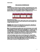
Scatter Graph, for Hypothesis 1
(On page 9)
The scatter graph shows the heights and weights of 60 different people. Scatter graphs are used to compare bivariate data. This graph is a very useful and effective, and it shows a pattern that, generally, as the height of a person increases, so does the weight. The line of best fit runs through the points, and shows how accurate my results are. There is a weak, but positive correlation on my graph. All the points were relatively close to the line of best fit, and the graph shows that there were no major anomalies in the data. The graph generally supports my first hypothesis.
Frequency Polygons and Histograms for boys and girls, for Hypothesis 2
(On pages 10 - 12)
The frequency polygons and the histograms were used to show the frequency and frequency density of different people’s IQs.
The frequency polygon for boys’ IQ shows that most boys that I picked randomly from my data, had an IQ between 100 and 105. The histogram, which is a more detailed version, tells us specifically, that most boys had an IQ between 100 and 103.
The frequency polygon for girls’ IQ, again, shows us that most boys had an IQ between 100 and 105, but the histogram tells us that the IQ was specifically between by 103 and 105.
The Line Graph, for Hypothesis 2
(On page 12)
The line graph shows the mean of both boys and girls IQ. It shows us, that from the data I picked, boys generally had a higher IQ than girls. This graph is a clear and effective one, supporting my second hypothesis well.
Histograms, for Hypothesis 3
(On pages 13 and 15)
The histograms were used in this hypothesis, to show the frequency density of boys in year 7 and 10 heights.
The histogram for year 7 boys’ heights shows that most boys have a height between 162 and 165.
The histogram for year 10 boys’ heights shows that most boys have a height between 173 and 175.
Cumulative Frequency Graphs and Box Plots, for Hypothesis 3
(On page 14, 16 and 17)
I did two cumulative frequency graphs fro year 7 and 10 boys’ heights. The cumulative frequency graphs show the median for both, and the results are the same as the ones from the histogram.
To present my results more clearly, I compared the two cumulative frequency graphs together.
To follow up on this, I did two separate box plots for each year group. The results show the minimum and maximum values, the median, and the upper and lower quartiles.
The Line Graph, for Hypothesis 3
(On page 17)
The line graph shows the mean of both boys in year 7 and year 10 heights.
It shows us, that from the data I picked, boys in year 10 generally have a higher average height than boys in year 7. This graph is a clear and effective one, supporting my third hypothesis well.
Evaluation
I can see that I have achieved fairly accurate results, in the first, second, and third hypothesis.
However, more evidence may have given me more even more reliable results. The raw data that I was given from Mayfield High School had many missing measurements and a few mistakes included in it, which may have affected results.
If I had collected the data myself, I could have corrected any faults and ensured reliability.
Applying these improvements to my investigation could improve the reliability.
Overall, I feel that I collected a sufficient amount of sample data, and my results support my three hypotheses.