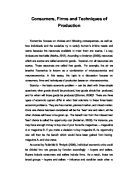
Sloman (2006) states, over a given period of time, resources are scarce, there is a limit to the amount of goods that can be made, and this can be shown using a graph (Figure 1) as followed:
Figure 1. The production possibility frontier
The curved line is called the production possibility frontier (PPF), other name for it includes production possibility curve. A PPF shows the maximum number of products that can be produced in an economy given its current level of resources (Anderton, 2008). Use apples and oranges as an example of production possibility, shown in Figure 2. Land is limited, if the number of apple trees decreased, there must be more oranges, and vice versa. In Figure 2, if there is 60 units of orange production only 75 units of apple can be produced. Thus, the opportunity cost of these 60 units of orange is 25 units (100 units – 75 units) of apple. The 75 units of orange have a lower opportunity cost: 15 units of apple. If the economy produces oranges only, the opportunity cost of the 100 units of orange goes to 60 units of apple.
Figure 2. The production possibility frontier and opportunity cost
Figure 3. Efficiency on the production possibility frontier
Every point shown in Figure 3 is efficient combinations of apples and oranges. In spite of A have 100 units of apple and no oranges, it is still efficient due to all resources are utilised.
Figure 4. Inefficiency on the production possibility frontier
In Figure 4, none of those points is efficient. Generally speaking, any points within the curve are inefficient. The reason is, there are also available resources have not been used (Threadgould & Meachen, 2008).
Figure 5. Shifts in the production possibility frontier
Points outside the curve are unlikely to be achieved by given current resources, but they are not cannot be reached forever. In Figure 5, if point A wants to shift to point B, it needs economic growth to increase available resources, and improvement in technology or increased skilled (Threadgould & Meachen, 2008). Also, a negative economy growth would lead to a shift in wards of the PPF, that is, from point B to point A. All of these movements and shifts will influence decision making. Production has been expanded through economic growth, for instance, then unemployment will decrease and firms need more employees to help them.
Figure 6. The production possibility frontier and marginal opportunity cost
Marginal opportunity cost is the gradient of the PPF. It means the opportunity cost from producing one more unit of a product. As Figure 6 shown, a concave PPF refers to increase in marginal opportunity cost, a convex PPF means a decreasing, and the straight downward sloping line means the marginal opportunity cost is constantly the same.
Threadgould & Meachen (2008) also states that, ‘firms aim to maximise profits’. It means the owners of firms want to maximise their return, based on this comes the better satisfaction of consumers’ needs and wants, the higher the potential for profit will be.
The factors of production are four components used to produce products, they are, land, labour, capital and enterprise (Anderton, 2008). Land means all naturally occurring resources whose location cannot be changed but use can be, such as actual land, copper and rivers. Labour is the workforce or labour force, it also called human effort. All manufactured resources used in production which can be separated into working and fixed capital -- that is, buildings, machinery, tools and vehicles – is known as capital, or physical capital. Enterprise means entrepreneurship; it requires people who are able to organise the first three components – land, labour and capital – into the productive process (Threadgould & Meachen, 2008). It could be called managerial ability. Four of them have their own type of reward, land earns rent, labour earns wages, capital earns interest, and enterprise earns profit.
Anderton (2008) believed that, demand is the ability and willingness to buy a good or service at a certain price over a period time. The demand curve can be plotted into a diagram shown on next page:
Figure 7. Demand curve
From the diagram above, Figure 7, we can know when the price is high, the quantity demanded is low, and vice versa.
Figure 8. Movements along the demand curve
Points on a demand curve refer to the quantity demanded at a certain price (Anderton, 2008). If there is a movement to the right ward, it means a decrease in the quantity demanded, and vice versa.
Figure 9. Shifts of the demand curve
Demand for the goods and services are talked about the entire curve (Anderton, 2008). It can be easily known that, an increasing in demand lead to a outwards shift of demand curve, and vice versa.
Owing to the concept of demand, there are several reasons to influence on demand, such as income, prices of other goods, advertising and changes in tastes. Threadgould & Meachen (2008) declared that, the higher the income, the higher the demand for normal goods. Normally, a good, for example, A, has substitutes and complements. A substitute, assumed as B, means a good can be used instead of A, such as Pepsi and Coca-Cola. If the price of B increases, the demand curve of A will shift to the right. A complement, assumed as C, means a good should be used with A, for instance, DVDs and DVD players. If the price of C increases, the demand curve of A will shift to the left because these two goods should be consumed together.
According to Rubinfeld & Pindyck (2009), supply is the quantity of goods that supplier are willing to sell at a given price. In a supply curve, inward shifts are occurred by non-price determinants, such as indirect taxation, costs of production and producer cartels. Outward shifts are caused by the development of new technology and subsidies. See Figure 10.
Figure 10. Shifts of the supply curve
In a brief, microeconomics presents an inter-relationship between buyers and sellers, consumers and firms, demand and supply, quantity and quality.
References
Anderton, A., (2008). Economics. 5th Edition. Essex: Pearson Education.
Pindyck, R.S. & Rubinfeld, D.L., (2009). Microeconomics. 7th Editon. New Jersey: Pearson Education.
Sloman, J., (2006). Economics. 6th Edition. Essex: Pearson Education.
Threadgould, A. & Meachen, A., (2008). Microeconomics for AS Level. Northumberland: Anforme Limited.