made on a given road. This includes
time costs, petrol costs and so on.
These total costs rise more than
proportionately with the number of
trips since, as more cars travel,
journey speeds are reduced,
increasing costs for a given trip.
This translates into the marginal
and average trip costs shown on Figure 2.2 by MC and AC respectively. The average cost
is the total cost divided by the number of trips, and the marginal cost is the cost of
making an additional trip from any particular existing total. Since total costs rise faster
than total trips, the marginal cost is always greater than the average cost – each extra trip
adds more to total costs than the previous trip.
At any point, the private cost to a motorist of making a trip is the average cost. If this
cost is less than the private benefit of the trip, the motorist will go ahead with the
journey. So the equilibrium number of trips occurs at the point where average costs equal
marginal benefits (as given by the demand curve, where we are assuming, as usual, that
demand decreases as price increases) – at point t0 in Figure 2.2. The socially optimal
number of trips would equate marginal benefits with marginal costs, leading to a lower
total number of trips, t. The optimal number of trips is lower than the private
equilibrium because each individual fails to take into account that, by undertaking a
journey, they slow down other road users, thereby adding to every user’s time and petrol
costs – a typical example of an externality. The social cost, or deadweight loss, associated
with this inefficient use of resources is shown by the shaded triangle in Figure 2.2. At
each point beyond t, the social costs of a trip exceed the benefits, and the deadweight
loss is the sum of these differences between t and t0.
If there are additional external costs, such as road damage costs or pollution costs, then
the true marginal social cost may be even higher than MC, such as the curve MC1 in
Figure 2.2. In this case, the optimal traffic volume is even lower, at t1.
In theory, there are several ways in which the relevant authorities could try to reduce the
traffic levels towards a more optimal level. Traffic bans could be imposed within the
specified area. Obviously, simply letting people turn up without knowing whether they
can enter is not a good idea, but there are other methods – in Athens, for example, cars
with odd or even number plates are banned on alternate days. Another option is to use a
price mechanism. The congestion problem arises because drivers are not faced with the
full costs of their actions, so an obvious solution is to make them pay these external
costs. In Figure 2.2, a charge per trip of c would effectively shift the average cost curve
up until it intersected the demand curve at t, leading to the efficient number of trips
being made. One advantage of using a congestion charge rather than a ban is that a
charge ensures that those drivers who value their journey least, or find it least costly to
change their behaviour, will forgo their car journey. To achieve a given reduction in
traffic in the most efficient way, we want the drivers with the lowest benefit from their
journey to alter their behaviour. A congestion charge makes sure that only those drivers
with a valuation of their journey (above the private costs already incurred) greater than or
equal to the charge continue to travel, whereas a ban based on number plates, say, would
not achieve the reduction so efficiently. Another obvious difference between restrictions
and charges is that a congestion charge raises revenue – shown by the rectangle ABCD in
Figure 2.2. This can be thought of as a straight transfer from motorists to the charging
authority, where it will then become part of public spending