Year 11 Girls
Year 11 Boys
In order to support my hypothesis, I will now carry out some analysis to my data. This will help me work out whether what I predicted was wrong or possibly right and supported. I will start by finding out the averages and measures of spread: the estimated mean, the modal class, the median class and the standard deviation to each year and then each gender from that year.
Year 7 girls
The modal class is 150.5≥h>160.5.
The median class is (33+1)/2 =17 which is 150.5≥h>160.5.
Estimated mean: 5109.25/33=154.83
Standard deviation:= 12.70 cm
Firstly worked out the modal class by seeing which group or class occurs most frequently. It turns out the modal class for Year 7 Girls is 150.5≥h>160.5. This shows me that the most popular heights for Year 7 girls are in that group.
I then followed on from that to work out the median class using the formula (n+1)/2. This showed me the “middle value, which happened to also be the class 150.5≥h>160.5. The median is a good way to work out the average when dealing with a set of numbers of which could be skewed by outliers.
Following on from that, I went on to find out the estimated mean. This is probably the most useful average, as it gives you the estimate of what the number is most likely to be. The estimated mean is 154.3 which lie between both the median and modal classes. These 3 averages would give me a really good insight into what I would predict as a year 7 girls height. The standard deviation shows me the average of the distance in between each piece of data. The standard deviation for year 7 girls was 12.70 cm. This is quite large deviation. This may be because the girls have different growth spurts in year 7, and extremely different growth rates due to puberty kicking in so there will be a huge variation.
I will now use a scatter graph, a cumulative frequency graph and a box plot to help analyse my data and then compare them to my hypothesis.
Scatter graph
The scatter graph shows two variables in one graph, and allows you to see what kind of correlation they have. There is a positive correlation between height and weight in the data, which supports my hypothesis greatly as I predicted this. However, within the scatter graph there are some plots that are slightly out the way of the main cluster. Due to the fact that humans are all different, and that all people develop differently and as this is year 7 girls, some girls may have already started their growth spurts towards adulthood and some may not have.
Cumulative Frequency graph
A cumulative frequency graphs shows the total running frequency of the data in a graph, and allows you do plot where the median and inter-quartile ranges are. The line of best fit on the year 7 girl’s cumulative frequency graph is flat and then all of a sudden steepens. This shows that after a certain point all the data is towards the higher end of my heights. This may suggest that some girls have not started puberty and not had their growth spurts, where as a lot of girls may have.
Year 7 boys
The modal class is 150.5≥h>160.5
The median class is (37+1)/2=16 which means 150.5≥h>160.5.
Estimated mean: 5678.5/37=153.47
Standard Deviation:= 7.96 cm
The modal class and the median class are exactly the same as the year 7 girls. This may be because in year 7, girls and boys work at different puberty rates so the difference between them isn’t as visible as in adults because the boys haven’t started developing yet. However, the standard deviation is very different from the girls. As this one is much lower than the other, this suggests that the girls are more wide-spread due to puberty. As boys generally start puberty later, there is a much less variety to the outside data, which is why there is less of an average distance difference between each piece of the data.
Scatter graph
The graph shows a positive correlation as I predicted in my hypothesis. Compared to the year 7 girls’ graph, it is a more definite positive correlation and there is less data lying outside the main cluster. This may be because the girls have started developing, and the boys may not have. Therefore the girls have more data lying outside the cluster as their puberty rates are all over the place but the boys may not have started.
Cumulative Frequency graph
The line of best fit on the cumulative frequency graph is smoother than the girls, this may be because, as I suggested before, the fact that the puberty rates for girls are quicker than the boys. This supports my hypothesis.
Scatter graph
The whole of year 7 data scatter graph shows yet again a positive correlation. Both girls and boys together from year 7 show that it is a close together cluster. This is showing that there is not much difference between the girls and boys in the main cluster. This may be because again of the puberty and that the outliers may be because the girls have started earlier than the boys.
Box Plot
Box plots or box and whisker diagrams are used to show the spread of the data, these diagrams show the highest and lowest value and the quartiles. The year 7 boys and girls box plots show that the interquartile ranges are very similar to each other, and are very close. However, the range of the box plot is huge with the girls, but much smaller with the boys. Yet again, this will be because the puberty rates of girls and boys are different as explained before. This supports my hypothesis greatly.
Year 11 girls
The modal classes are 155.5≥h>160.5, 160.5≥h>165.5 and 165.5≥h>170.5.
The median class is (22+1)/2=11.5 which is 160.5≥h>165.5.
Estimated mean: 3515.75/22=159.81
Standard deviation:= 9.36 cm
For year 11 girls, there are three modal classes. They are also all in order, 155.5≥h>160.5, 160.5≥h>165.5 and 165.5≥h>170.5. The median class is 160.5≥h>165.5, which is the middle one out of the modal classes. The estimated mean is 159.81 which is higher than the year 7 girls and boys, which is understandable because as people get older during teenage years they grow. The standard deviation is much less than that of the year 7 girls, as it is 9.36. This may imply that the girls have almost finished puberty, or have finished in some cases possibly.
Scatter Graph
This is again a positive correlation, and supports my hypothesis. However, due to the 25% of data I used from each year, it’s harder to see than any of the year 7 data. There is a cluster but it’s more spread out than the year 7 data, which is probably closer together due to the puberty rates. However, in the year 11 girls scatter graph there is only one piece of data away from the main cluster, but in the year 7 girls scatter graph there was numerous pieces, possible due to the puberty rates again. This supports my hypothesis, and lets me explore deeper into it.
Cumulative Frequency graph
The cumulative frequency graph shows that the year 11 girls’ heights have quite and eased line of best fit compared to the year 7 girls graph which was all of a sudden quite steep. This is probably because the puberty levels have eased out.
Year 11 Boys
The modal class is 175.5≥h>195.
The median class is (21+1)/2 which is 165.5≥h>170.5.
Estimated mean: 3589.5/21=170.93
Standard deviation:= 12.36 cm
The immediate thing I notice about the year 11 boys’ data is that the outcomes from are much higher than any other set of data within this. The modal class is 175.5≥h>195 whereas with year 7 boys and girls and year 11 girls were between 155.5≥ h>170.5 between all the data. The boys in year 11 will be possibly higher due to the fact that year 11 boys are closer to adulthood than they were in year 7, therefore starting to take on their fully grown height. The estimated mean is large as well, much higher than the year 11 girls whereas in year 7, both girls and boys data outcomes seem to have been much closer if not almost identical. However, the standard deviation is quite high, which shows that some boys may not be going through full puberty yet.
Scatter graph
Again, the boys scatter graph definitely has a positive correlation which supports my hypothesis. It is far higher up the scale than the year 7 boys though, which possibly means that they are getting more developed to how they are meant to be as adults. Compared to the girls it is clearer from the correlation, but has more outliers.
Cumulative Frequency
The line of best fit for year 11 Boys is very curvy compared to the other cumulative frequency graphs. It is more subtle but it curvy towards the lower values whereas the others were far steeper. This may be because all the boys have almost completely evened out, as they start puberty later and finish earlier than girls. This supports by hypothesis.
Scatter Graph
Compared to the year 7 pupils’ graph, the correlation of year 11 pupils is still positive but is less distinct. This may be due to the fact that year 11 pupils have started to get their own body shape and height and are turning into adults, but the years 7’s still have puberty to hit although some may have already started to hit it.
Box Plot
The year 11 box plot has a distinct difference between the girls and boys, the boys range is around the same as the girls range but the boys’ box plot is far higher up the scale than the girls. This is possibly because the boys are starting to fully develop, and as are the girls so they are almost in their adult form. At adult stage, boys are normally the taller which suggests why the year 11 box plot is like that.
Conclusion
In conclusion, all of my findings have been helpful and almost all support my hypothesis. I think the amount of data I used was helpful, but would have been much more accurate if I’d have taken a larger sample, because the larger the sample the more accurate your findings become because you cover more. If I were to do it again, I may want to take 30 – 40 % of students from each year, instead of the initial 25 % I used. I would also include other years in my sample, so investigate how it would progress and possibly increase my variety of showing data, i.e. histograms and using spearmen’s rank. I would also consider taking out more outliers to make sure my end results weren’t skewed or anything by them and then maybe look at the data as a whole without grouping it first, to make it even more accurate. However, this is very time consuming. The approach I had in my hypothesis got supported the whole way through my findings – which height and weight had a positive correlation and that puberty affected the rates so that year 7 would be different to year 11 and that girls would be different to boys. I have found that the data I had suggests that the older you get, the more stable the heights and weights become, and they are not so all over the place and the clusters are tighter the older you get. I also found that the data suggests that in year 7 girls, there is a wider range compared to year 7 boys. This could be because of the puberty rates. By the time we get to the year 11 data, both girls and boys are pretty stable, of course there are some slightly off-the-cluster data, which is normal due to no human being is the same. All in all, what I have discovered is that my findings support my hypothesis, but if I were to investigate this again, I would do some things slightly differently, but some things I would keep very much the same – after all my data did support what I predicted in the first instance.