a = Acceleration
v = Final Velocity
u = Initial Velocity
s = Distance
t = Time
- a = (v-u)/ t
-
v2 = u2 + 2as
-
s = ut + ½at2
- s = ½(v + u)t
- v = u + at
As well as this I can use Newton’s Second Law to Model the Particle, in order to find out friction etc.
Newton’s second law states, ‘The Force, F, applied to a particle is proportional to the mass, m, of the particle and the acceleration produced.’
This can then be represented by the equation F=ma
In order to model the trolley I must know the acceleration. I will therefore use the SUVAT equations first.
Using the SUVAT equations
Firstly I will calculate the velocity of the card through the light gate using the formula:
(First Light Gate)
Speed = Distance / Time
= 0.03 / 0.15544 (the card is 3cm long = 0.03m)
= 0.193
I will now do this for all the light gate positions.
Next I shall work out the time for the card to reach the light gate by rearranging the equation:
S = ½ (v + u)t
Therefore 2s = (v + u)t
T = 2s / v (as initial velocity is always zero)
Therefore for the first light gate the trolley takes:
T = 0.2 / 0.193
= 1.03s
I can now do this for all the other light gate positions also.
I can now work out the acceleration of the trolley through the light gate by using the formula:
A = (v – u) / t
For the first light gate
A = 0.193 / 1.03
= 0.186ms-2
I will now apply this equation for all the other light gate positions.
Now that I have acceleration for the trolley I can model it as a particle going down a slope and find out the model acceleration. This value can then be subtracted from the actual value to give resistance to the path of the trolley.
Modelling the Trolley
The Trolley can be modelled as a right angle triangle and thus further information can be found out such as the angle of the slope and then consequently the friction can be found out.
122cm
2.5cm
Angle θ
Working out the angle
If Sin θ = 2.5/122
Therefore θ = sin-1 (2.5/122)
= 1.17*
Therefore the angle of the slope is 1.17 degrees.
Using this I can now work out what the acceleration of the model is. This should be greater than the values I obtained using the SUVAT formulas as I am not taking into account friction etc.
R
μN
Mgsinθ
Perpendicular to the Slope : Mgcosθ = R
(0.623 x 9.8) cos 1.17 = N
Therefore R = 6.104N
I can now calculate the friction along the slope at various distances down the slope. This is the overall resistance to the driving force of the trolley, so can include air resistance.
Along the Slope: F = Mgsinθ - μR where F is total driving force
At 0.1m down slope ma = Mgsinθ - μR
- = 0.125 – 6.104μ
8.6 x 10-3 = 6.104μ
Therefore μ = 1.41 x 10⁻³
At 0.8m down the slope F = Mgsinθ – μR
Ma = Mgsinθ – μR
0.095 = 0.125 – μ6.104
0.03 = 6.104μ
Therefore μ = 5 x 10⁻³
Using this formula I have calculated the friction for all the other distances and is shown in the results table.
As well this I can calculate the gravitational potential energy and the kinetic energy. I will then be able to take the kinetic energy away from the gravitational potential energy to work out the energy lost in the form of sound, heat etc. Below is shown two examples of each.
Kinetic Energy = ½mv2
At 0.1m down the slope: KE = ½ x 0.623 x 0.1932
= 0.0116J
At 0.8m down the slope: KE = ½ x 0.623 x 0.2672
= 0.0222J
Gravitational Potential Energy = Mass x Velocity x Height
In order to work out the gravitational potential energy I must use trigonometry to calculate the height of the trolley at certain light gates. For simplicity only two examples are shown below. The others are shown in the results table later on.
At 0.1m down the slope:
112cm
x
Angle θ = 1.17 degrees
If sin θ = x / 112
Then x = 112 sin θ
= 2.29cm (2d.p.)
Therefore I can now calculate the gravitational potential energy of the trolley at the first light gate.
GPE = Mass x Gravity x Height (in metres)
= 0.623 x 9.8 x 0.0229
= 0.140J
At 0.8m down the slope:
42cm
y
Angle θ = 1.17 degrees
If sin θ = y / 42
Then y = 42 sin θ
= 0.86cm (2 d.p.)
Therefore GPE = Mass x Gravity x Height
= 0.623 x 9.8 x 0.0086
= 0.053J
Sources of Error
Measuring the distance from where the trolley is released was a source of error in the experiment. If the trolley was released slightly in front or behind from where it should have been released from, this would cause the time for the card to pass through the light gate to differ.
As well as this the card may have hit the light gate causing it to drastically slow down and therefore cause the time taken for it to pass through the light gate to increase. This would further have an impact on the rest of the experiment because the shape of the card may have been modified upon collision-
E.g. initially the length of the card which the light gate is measuring would be 3cm. If, however, it then crashes, the shape of the card would be distorted. The point at which the light gate is measuring the time for the card to pass through the light gate may then increase as the card has crumpled and so it longer in length and vice versa.
We must also consider the fact that at some point the slope may have slightly slipped, causing the gradient of the slope to change. This would obviously greatly affect the rate of acceleration of the trolley and produce inaccurate results.
There are therefore many sources of error in this procedure which must be accounted for in the experiment.
The results from my experiment are shown in the tables in the following pages, as well as explanations of the graphs I have drawn.
Analysis
Graph 1: Comparing Actual Velocity of Trolley as it goes down the slope
From the graph you can see that as the trolley goes down the hill it picks up speed. The greatest change increase in velocity occurs at the top of the slope and can be described due to the fact that at this point is has the most GPE to convert to KE.
As the trolley goes down the slope, however, it is clear that the velocity increase is not proportional to the distance it travels. This can be accounted for due to the friction I have calculated. However this remains constant so there must be another factor involved. It must therefore be air resistance as this increases as you go faster. Therefore as the trolley picks up speed, it is slowed down more until it reaches its terminal velocity.
I chose to do this graph as it is a visual aid in seeing how the trolley changes in speed through its course.
Graph 2: Graph showing how the long it takes for the trolley to go down the slope to various distances
The graph shows an almost proportional trend in that as the distance increases so does the time it takes for the trolley to go this distance. There is however a slight curve towards the end. This can be accounted for in that the trolley has more air resistance as it goes down the slope, so the time it takes must increase. Therefore the rate must slow, so the graph starts to level out. However it seems that the trolley reaches its terminal velocity reasonably quickly as the rate is almost constant.
Graph 3: Graph showing how the Kinetic Energy of the trolley changes as it goes down the slope
The graph shows as that as the trolley goes further down the slope, its kinetic energy increases. This is very easy to explain in that as it moves down the slope it picks up more speed. The equation for kinetic energy is KE = ½mv2. The mass of the particle does not change and so the rise in kinetic energy is solely due to the trolley increasing in speed. When it is higher up the slope, it has more gravitational potential energy so it can not posses as much kinetic. Lower down the slope it has less GPE so it can posses more KE.
Graph 4: Graph to show how the Gravitational Potential Energy of the trolley changes as it goes down the slope
The graph shows that as the trolley goes further down the slope it has less gravitational potential energy. This is also easy to explain in that when it is at the top of the ramp it has more height. Since GPE = mgh, the more height it has the more GPE it shall have. As it moves down the slope it is not as high up, so it has less GPE.
Graph 5: Comparing GPE with KE
This graph basically illustrates the connection between GPE and KE. It shows that when one increases the other must decrease. Using this graph and plotting interpolation lines and then using the GPE against distance graph one can work out the position of the trolley at a given location.