Therefore,
y = (-2 x 10⁻⁵)x + 2.2
Here, the variable y can be replaced by rn which represents the growth factor at some year n and the variable x can be replaced by un which represents the population at some year n. Therefore, the equation for the linear growth factor in terms of un will be: -
rn = (-2 x 10⁻⁵)un + 2.2
Now, to find the recursive logistic function, we shall substitute the value of rn calculated above in the following form un+1= rn.un
un+1 = [(-2 x 10⁻⁵)un + 2.2]un
= (-2 x 10⁻⁵)un2 + 2.2un
To find out the changes in the pattern, let us see the following table which shows the first 20 values of the population obtained according to the logistic function un+1= (-2 x 10⁻⁵)un2 + 2.2un just calculated: -
The above tabulated data is represented by the following logistic function: -
Here, from the table and graph we can observe how the population rapidly grows beyond the sustainable limit (which is 60,000) to 60440 within 4 years itself but then comes down below 60000 to 59907 in the successive year. Such an increasing and decreasing trend in the population is observed in the following years although the population seems to come closer to the sustainable limit, i.e 60000 all the time. In the 8th year, the population is exactly at its sustainable limit and henceforth, the population stabilizes by only varying slightly until the 18th year.
-
when the initial growth rate r0 = 2.3
The ordered pair (u0, r0) for the first pair when the predicted growth rate ‘r’ for the year is 2.3 will be (10000, 2.3).
(un, rn) = (60000, 1) according to the description.
We can get the equation of the linear growth factor by entering these sets of ordered pairs in the STAT mode of the GDC Casio CFX-9850GC PLUS.
The STAT mode looks as follows: -
Thus, we obtain a linear graph which can be modeled by the following function: -
y = (-2.6 x 10⁻⁵)x + 2.56
Here, the variable y can be replaced by rn which represents the growth factor at some year n and the variable x can be replaced by un which represents the population at some year n. Therefore, the equation for the linear growth factor in terms of un will be: -
rn = (-2.6 x 10⁻⁵)un + 2.56
Now, to find the recursive logistic function, we shall substitute the value of rn calculated above in the following form un+1 = rn.un
un+1 = [(-2.6 x 10⁻⁵)un + 2.56]un
= (-2.6 x 10⁻⁵)un2 + 2.56un
To find out the changes in the pattern, let us see the following table which shows the first 20 values of the population obtained according to the logistic function un+1= (-2.6 x 10⁻⁵)un2 + 2.56un just calculated: -
The above tabulated data can be represented by the following logistic function graph: -
Again, the table and graph show how an initial growth rate of more than 2 makes the population grow rapidly beyond the sustainable limit (which is 60,000) to 62577 within 3 years which is more rapid and higher than when the growth rate is 2. In the successive year, the population falls to 58384 yet it again rises in the next year. Such a trend of increase and decrease in the population goes on till the 17th year. Also as a result of a higher initial growth rate, it takes more time for the population to become stable at the sustainable limit of 60,000. This is reached in the 17th year.
-
when the initial growth rate, r0 = 2.5
The ordered pair (u0, r0) for the first pair when the predicted growth rate ‘r’ for the year is 2 will be (10000, 2.5).
(un, rn) = (60000, 1) according to the description.
We can get the equation of the linear growth factor by entering these sets of ordered pairs in the STAT mode of the GDC Casio CFX-9850GC PLUS. The STAT mode looks as follows: -
Thus, we obtain a linear graph which can be modeled by the following function: -
y = (-3 x 10⁻⁵)x + 2.8
Here, the variable y can be replaced by rn which represents the growth factor at some year n and the variable x can be replaced by un which represents the population at some year n. Therefore, the equation for the linear growth factor in terms of un will be: -
rn = (-3 x 10⁻⁵)un + 2.8
Now, to find the recursive logistic function, we shall substitute the value of rn calculated above in the following form un+1 = rn.un
un+1 = [(-3 x 10⁻⁵)un + 2.8]un
= (-3 x 10⁻⁵)un2 + 2.8un
To find out the changes in the pattern, let us see the following table which shows the first 20 values of the population obtained according to the logistic function un+1= (-3 x 10⁻⁵)un2 + 2.8un just calculated: -
The above tabulated data can be represented by the following logistic function graph: -
The table and graph confirm how higher growth rates above 2 lead to less stability in population. Here, the variance from the long term sustainable limit (which is 60000) is much more (64703 in the 3rd year) compared to when the initial growth rate was 2.3 or 2. The successive year sees a similar larger fall to 55573 in population compared to the other two cases. Consequently, the table confirms how a high initial growth rate leads to longer time for the population to stabilize at the long term sustainable limit. In this case, it is not attained in the first 20 years. Rather, upon further calculations we can find out that the population becomes stable at the long term sustainable limit in the 41st year compared to the 17th year when the initial growth rate is 2.3 .
Part 5
Let us see what happens when the initial growth rate is 2.9
The ordered pair (u0, r0) for the first pair when the predicted growth rate ‘r’ for the year is 2 will be (10000, 2.9).
(un, rn) = (60000, 1) according to the description.
We can get the equation of the linear growth factor by entering these sets of ordered pairs in the STAT mode of the GDC Casio CFX-9850GC PLUS.
Thus, we obtain a linear graph which can be modeled by the following function: -
y = (-3.8 x 10⁻⁵)x + 3.28
Here, the variable y can be replaced by rn which represents the growth factor at some year n and the variable x can be replaced by un which represents the population at some year n. Therefore, the equation for the linear growth factor in terms of un will be: -
rn = (-3.8 x 10⁻⁵)un + 3.28
Now, to find the recursive logistic function, we shall substitute the value of rn calculated above in the following form un+1 = rn.un
un+1 = [(-3.8 x 10⁻⁵)un + 3.28]un
= (-3.8 x 10⁻⁵)un2 + 3.28un
To find out the changes in the pattern, let us see the following table which shows the first 20 values of the population obtained according to the logistic function un+1= (-3 x 10⁻⁵)un2 + 2.8un just calculated: -
The above tabulated data can be represented by the following logistic function graph: -
We can infer from the data in the table and the graph how a high initial growth rate of 2.9 can lead to fluctuating populations every year. The long term sustainable limit of 60,000 is crossed at the end of the 2nd year itself, becoming 63162. But, in such a case, the environment (in this case the lake) cannot withhold such a population and thus there are a lot of fishes either dying out or migrating in the subsequent year which reduces the population to 55572. Yet, again in the next year, due to high growth rate, the population reaches well above even 63162 to 64922. Such a fluctuating trend is observed in the succeeding years until the end of the 16th and 17th year during and after which the population fluctuates between 70719 and 41911.
Part 6
To initiate an annual harvest of 5000 fishes, let us first find out at what point the fish population stabilizes when the initial growth rate, r = 1.5.
The following table shows the growth in the population over the first 20 years taking r = 1.5 and thus making use of the following recursive relation as found out in Part 2:-
un+1 = (-1 x 10⁻⁵) un2 + 1.6un
In this relation, the starting population is the initial population u0 = 10000.
Here, we see that the population reaches a stable point, when r =1 at the end of the 16th year. According to the question, we shall initiate the harvest of 5000 fishes every year from this point onwards. The following changes are made in the original recursive relation:-
- The starting population is taken to be 59999
-
In the relation un+1 = (-1 x 10⁻⁵) un2 + 1.6un , we subtract 5000 as this is the number which is removed every year. Thus, the new relation becomes
un+1 = (-1 x 10⁻⁵) un2 + 1.6un – 5000
It should be noted that although the start population or u0 is taken to be 59999, the starting year is the 16th year.
Entering these values in the RECUR mode of the GDC Casio CFX 9850GC Plus, we get the following table:-
We see that there is a declining trend in the fish population with an annual harvest of 5000 fishes when the growth rate is 1.5. However, it should be noted that with this annual harvest, the population finally stabilizes in the 34th year when it becomes 50000.
The graph is as follows: -
Thus, we can conclude that it is feasible to initiate an annual harvest of 5000 fishes once the stable population of 59999 is reached in the 16th year with the growth rate being 1.5.
Initially, a declining trend in the fish population is observed as 5000 fishes are harvested every year. Yet, from the 34th year onwards, we observe that the new stable fish population becomes 50,000 with an annual feasible harvest of 5000 fishes.
Part 7
Taking the same model in which the growth rate r = 1.5, we shall investigate other harvest sizes.
- When the harvest size = 2500 fishes
We shall initiate the harvest of 2500 fishes after the 16th year when the population stabilizes at 59999. The following changes are made in the original recursive relation:-
- The starting population is taken to be 59999
-
In the relation un+1 = (-1 x 10⁻⁵) un2 + 1.6un , we subtract 2500 as this is the number which is removed every year. Thus, the new relation becomes
un+1 = (-1 x 10⁻⁵) un2 + 1.6un – 2500
Entering these values in the RECUR mode of the GDC Casio CFX 9850GC Plus, we get the following table:-
The graph is as follows: -
We see that when the annual harvest is 2500, there is a declining trend which stabilizes quite early, that is from the 28th year onwards compared to when the harvest is 5000 fishes. Also, the new stable population, 55495 is higher compared to when the harvest if 5000 fishes.
Thus, we can conclude that it is also feasible to initiate an annual harvest of 2500 fishes and the new stable population would be achieved from the 28th year onwards as 55495.
- When the harvest size = 7500
We shall initiate the harvest of 7500 fishes after the 16th year when the population stabilizes at 59999. The following changes are made in the original recursive relation:-
- The starting population is taken to be 59999
-
In the relation un+1 = (-1 x 10⁻⁵) un2 + 1.6un , we subtract 7500 as this is the number which is removed every year. Thus, the new relation becomes
un+1 = (-1 x 10⁻⁵) un2 + 1.6un – 7500
The table settings are as follows: -
Entering these values in the RECUR mode of the GDC Casio CFX 9850GC Plus, we get the following table:-
The graph is as follows: -
The above table and graph show that when the harvest is as high as 7500, the population has an increasing decreasing trend compared to when the harvest size is 5000. Also, the population does not seem to stabilize by the 35th year. By further investigating, the stable population is found to be in the 55th year.
Thus we can conclude that it is also feasible to initiate an annual harvest of 7500 fishes even though the stable population is lower than when the harvest size is 5000.
- When the harvest size = 4000 fishes
We shall initiate the harvest of 4000 fishes after the 16th year when the population stabilizes at 59999. The following changes are made in the original recursive relation:-
- The starting population is taken to be 59999
-
In the relation un+1 = (-1 x 10⁻⁵) un2 + 1.6un , we subtract 4000 as this is the number which is removed every year. Thus, the new relation becomes
un+1 = (-1 x 10⁻⁵) un2 + 1.6un – 4000
Entering these values in the RECUR mode of the GDC Casio CFX 9850GC Plus, we get the following table:-
The graph is as follows: -
The above table shows that when the harvest is 4000, the population has a less decreasing trend compared to when the harvest size is 5000. Also, the population stabilizes by the 33rd year, an year earlier than when the harvest size is 5000.
Thus we can conclude that it is also feasible to initiate an annual harvest of 4000 fishes and the stable population is higher than when the harvest size is 5000.
- When the harvest size = 10000 fishes
We shall initiate the harvest of 10000 fishes after the 16th year when the population stabilizes at 59999. The following changes are made in the original recursive relation:-
- The starting population is taken to be 59999
-
In the relation un+1 = (-1 x 10⁻⁵) un2 + 1.6un , we subtract 10000 as this is the number which is removed every year. Thus, the new relation becomes
un+1 = (-1 x 10⁻⁵) un2 + 1.6un – 10000
The table settings are as follows: -
Entering these values in the RECUR mode of the GDC Casio CFX 9850GC Plus, we get the following table:-
The graph is as follows: -
The above table and graph shows that when the harvest is as high as 10000, the population has an increasing decreasing trend compared to when the harvest size is 5000 or even 7500. The population does not stabilize at all, and in fact, dies out by the 42nd year when the value as shown by the calculator is -2150, and when the curve crosses or cuts the x-axis, indicating that the population is extinct or has died out.
Thus we can conclude that it is not feasible at all to initiate an annual harvest of 10000 fishes.
Part 8
We shall use the ‘Hit and Trial’ method to find out the maximum annual sustainable harvest by examining different harvest sizes: -
The same methods shall be employed as in Part 7 for different harvest sizes, that is: -
- The starting population is taken to be 59999
-
In the relation un+1 = (-1 x 10⁻⁵) un2 + 1.6un , we subtract x which is the harvest size taken in the particular case and is removed every year. Thus, the new relation becomes
un+1 = (-1 x 10⁻⁵) un2 + 1.6un – x
-
We start by taking the harvest size, x = 7500
The new recursive function becomes un+1 = (-1 x 10⁻⁵) un2 + 1.6un – 7500 which we shall enter in the RECUR mode of the GDC Casio CFX-9850GC Plus. We have used the same table range as in Part 7.
As found out already in Part 7, the population stabilizes in the 52nd year at 42247.
Thus, there is scope for a higher harvest.
-
Next, we take the harvest size, x = 8500
The new recursive function becomes un+1 = (-1 x 10⁻⁵) un2 + 1.6un – 8500 which we shall enter in the RECUR mode of the GDC Casio CFX-9850GC Plus.
The graph is as follows: -
It is observed that the population stabilizes from the 75th year at 37071.
We can try further higher values.
-
When the harvest size, x = 9500
The new recursive function becomes un+1 = (-1 x 10⁻⁵) un2 + 1.6un – 9500 which we shall enter in the RECUR mode of the GDC Casio CFX-9850GC Plus. The table settings are: -
The graph is as follows: -
From the graph we see that the curve crosses or cuts the x-axis which indicated that the population dies out or becomes extinct during the 54th year.
Therefore, we should try lower values.
-
When the harvest size, x = 8900
The new recursive function becomes un+1 = (-1 x 10⁻⁵) un2 + 1.6un – 8900 which we shall enter in the RECUR mode of the GDC Casio CFX-9850GC Plus. The table settings are as follows: -
The graph is as follows: -
It is observed that the population becomes stable only after the 150th year.
We can try slightly higher values.
-
When the harvest size, x = 9100
The new recursive function becomes un+1 = (-1 x 10⁻⁵) un2 + 1.6un – 9100 which we shall enter in the RECUR mode of the GDC Casio CFX-9850GC Plus. The table settings are as follows: -
The graph is as follows: -
It is observed that the population dies out and becomes extinct during the 109th year.
Thus, the maximum sustainable harvest size must be somewhere between 8900 and 9100.
-
Let us try with the harvest size, x = 9000
The new recursive function becomes un+1 = (-1 x 10⁻⁵) un2 + 1.6un – 9000 which we shall enter in the RECUR mode of the GDC Casio CFX-9850GC Plus. The following are the table settings: -
The graph in the range 700th and 800th year is as follows: -
Let us also see some of the table values in this range: -
These values show that the population is decreasing in this range but at a very slow rate. Therefore, let us see whether the population becomes extinct during the 1700th and 1800th year:-
Also, some of the table values in this range are: -
The graph and these values above again show that the population is more or less stable between high years between the 1600th and 1700th year.
It is seen that the population does not die out even beyond the 1700th year or so. Moreover, the rate of decreasing of the population keeps on decreasing. Hence, we can assume that the population eventually becomes stable.
- To prove that 9000 is the maximum annual sustainable harvest, we shall check whether
the population dies out or not when the harvest size, x = 9001
The new recursive function becomes un+1 = (-1 x 10⁻⁵) un2 + 1.6un – 9001 which we shall enter in
the RECUR mode of the GDC Casio CFX-9850GC Plus. The table settings are as follows: -
The graph between the 1st year and the 100th year is as follows: -
The following graph shows the values from the 950th to 990th year: -
The population is found to die out during the 1003th year which proves that 9000 is the maximum sustainable harvest which is possible.
Part 9
Using the first model, that is, with the initial fish population of 10000, we shall determine whether it will be feasible to harvest immediately from the 1st year with different harvest sizes: -
-
Let us start by taking the maximum sustainable harvest of 8000 (as calculated in Part 8) and check whether it is feasible to start harvesting from the 1st year itself.
The new recursive relation will be un+1 = (-1 x 10⁻⁵) un2 + 1.6un – 8000
We set the following range for the table:
Entering the values in the RECUR mode of the GDC Casio CFX-9850 GC Plus, we get the following table: -
The table and graph show how the population dies out or becomes extinct during the 3rd year and thus it would not be economically beneficial with a harvest size of 8000.
- Let us try with a lower value such as 6500
The new recursive relation will be un+1 = (-1 x 10⁻⁵) un2 + 1.6un – 6500
We set the following range for the table:
Entering the values in the RECUR mode of the GDC Casio CFX-9850 GC Plus, we get the following table: -
Again the table and the graph show how the population dies out during the 4th year proving that it will not be beneficial.
- Let us try with further lower value such as 5000.
The new recursive relation will be un+1 = (-1 x 10⁻⁵) un2 + 1.6un – 5000
We set the following range for the table:
Entering the values in the RECUR mode of the GDC Casio CFX-9850 GC Plus, we get the following table: -
Hence we see that the population sustains from the 1st year of harvest itself.
To check whether 5000, is the maximum harvest that can be done from 10,000 so that the population sustains faster, we can take a slightly higher value and check whether that will be sustainable.
The new recursive relation will be un+1 = (-1 x 10⁻⁵) un2 + 1.6un – 5001
We set the following range for the table: -
Entering the values in the RECUR mode of the GDC Casio CFX-9850 GC Plus, we get the following
table: -
The graph and table shows how the population dies out during the 25th year itself. Thus, even 5001 is not sustainable.
-
We start by taking the initial population size = 10000 fishes and initiating a harvest of 8000 fishes from the 1st year itself.
The new recursive function becomes un+1 = (-1 x 10⁻⁵) un2 + 1.6un – 8000. Also, the starting population, u0 = 10000. This shall be entered in the GDC Casio CFX-9850GC Plus.
In this case, we find out that the population dies out during the 3rd year which means that such a combination is not sustainable.
-
Let us increase the initial population size = 16000 fishes and initiate a harvest of 8000 fishes from the 1st year itself.
The new recursive function becomes un+1 = (-1 x 10⁻⁵) un2 + 1.6un – 8000. Also, the starting population, u0 = 16000. This shall be entered in the GDC Casio CFX-9850GC Plus.
In this case also, we find that the population dies put during the 7th year which means that such a combination also is not sustainable.
-
Let us try with an initial population size of 19000 fishes and initiate a harvest of 8000 fishes from the 1st year itself.
The new recursive function becomes un+1 = (-1 x 10⁻⁵) un2 + 1.6un – 8000. Also, the starting population, u0 = 19000. This shall be entered in the GDC Casio CFX-9850GC Plus.
The graph and GDC show that the population dies out during the 14th year which means that this combination is not sustainable.
-
When the initial population size is 20000 fishes and a harvest of 8000 fishes is initiated from the 1st year itself.
The new recursive function becomes un+1 = (-1 x 10⁻⁵) un2 + 1.6un – 8000. Also, the starting population, u0 = 20000. This shall be entered in the GDC Casio CFX-9850GC Plus.
Using this combination, we have found out using the GDC that the population remains constant and stable starting from the 1st year itself. It neither depletes nor increases. Thus, this introductory fish population size of 20000 is the most sustainable for harvesting 8000 fishes.
-
To prove that an initial population of 20000 fishes is the most suitable and sustainable for a harvest of 8000 fishes every year, we shall investigate using u0 = 19999.
The new recursive function becomes un+1 = (-1 x 10⁻⁵) un2 + 1.6un – 8000. Also, the starting population, u0 = 19999. This shall be entered in the GDC Casio CFX-9850GC Plus.
The GDC shows that in such a case, the population has a decreasing trend which slowly increases with increasing number of years and finally, dies out during the 52nd year. Hence, an initial population size of 19999 is not sustainable.
These results help us to infer that a minimum initial population size of 20000 fishes is required to sustain a harvest of 8000 fishes every year from the 1st year.
Candidate Name: - Sanchit Ladha
Candidate Session No.: -1070-006