“Where σ²p is the variance of return on a risky portfolio; wA is the value-weighted proportion of a portfolio invested in asset A; σ²Α is the variance of the rate of return in asset A; wB is the value weighted proportion of a portfolio invested in asset B; σ²B is the variance of the rate of return on asset B; and pAB is the correlation coefficient of returns between asset A and asset B.”(Keith Pilbeam, finance & financial markets, published 1998, page 131).
By using this type in an example where a portfolio has two securities A and B we can observe that diversification has a role in reducing the risks facing an investor. However, it cannot reduce the expected reduce which is the return on the individuals financial assets. Therefore, it is easy to understand that diversification is about reducing the variability of return and not only a mean of enhancing the return on a portfolio.
When the returns on securities A and B have different degrees of correlation, we can view three extreme cases that happen to the variability of return. First when there is perfect positive correlation (pAB=1), from portfolio diversification there are no gains. Next case is when there is perfect negative correlation (pAB=-1), the profits from portfolio diversification are at a highest level. In the last case where there is zero correlation (pAB=0), the profits are not as big as in the case of perfect negative correlation.
Every risk-averse investor puts as target to minimize the risk of a given return, so he would try to choose a weighted combination, which will help him to achieve that. The way that we can see when a combination of two risky shares has a maximum rate of return for a given level of risk, or those with the minimum rate of risk for any given rate of return, is the so called efficiency frontier. Also the investor has unlimited number of investment opportunities in allocating his wealth between securities A and B and the mapping of this potentials gives the mean-variance.
However, in fact, investors in reality must make their choice from a larger range of risky assets. It is easily understood that there can be an extremely big number of possible portfolios that have different asset mixes from which they must choose. If we assume that we have N different assets, we can have numerous possible portfolios that contain different mixes of assets that could be constructed. The following graph will show the map of all the portfolios that could be created with N assets.
GRAPH 1
Expected
return
E
A
B D
C
F
Risk/standard deviation
When a portfolio dominates another, it will happen because either it has the same standard deviation, or it has a lower standard deviation and the same expected rate of return as another portfolio, and this is called the dominance principle. We can read from the graph that portfolio A dominates B and B dominates C and D. But not all combinations are of interest since some of them dominate others. In this case, we can see that A dominates C and E dominates portfolio F, so our attention focuses only in the thick black part of the efficiency frontier. The portfolios that dominates the others portfolios is the so-called efficiency frontier. Furthermore, all dominated portfolios are called inefficient portfolios and the portfolio that for a given level of risk offers the highest possible return is called efficient portfolio.
A technique, which is known as quadratic programming, and comes from the Markowitz method, can give us the mathematical solution for the portfolio efficiency frontier. The basic ingredient in this technique is to calculate a reachable target rate of return X% and then find a set of weights wi, which attains this target with the minimum of variance, which is illustrated next:
N N N
σ²p=Σw²i σ²i +Σ Σ wi wj σij
I=1 I=1 I=1
i =j
Then by using the diversification, the risk can be reduced until the minimum risk of a given return is reached. This can be achieved by minimizing the correlation among the rates of return on two or more securities. However, this method has a major problem, which has to do with the amount of covariances that have to be calculated. In N securities the formula that is used is (N²- N)/2 and we think of 500 securities then the covariances goes over the number of 120.000. but even in N securities the risk of every combination will be less than the weighted average of the securities that make up the portfolio.
While the risk can be reduced through diversification, providing that returns are not either positively or negatively and perfectly correlated, it is not able to remove every risk attached to an asset, which is inherent in the market. Specific risk is the risk that can be eliminated by diversification while market risk is the one that is attached to an asset cannot be eliminated by the diversification as we can see from the following graph (graph 2). GRAPH 2
If an investor wanted to construct a portfolio from N securities then would have two choices. He would make a choice between portfolios either with all or with less than N securities. In order to find out how many securities he would choose, we have to use a process called naïve diversification. According to that process, we have to take randomly a variety of shares that there is no possible correlation between them. An example of that method is the investigation of the issue of UK securities that he made. All the selections were made randomly, of size among 1 and 50 shares and the average risk a percentage of the average risk of keeping only one share when estimated. The results showed that the profits of desertification in terms of risk decrease are rather extensive up to 20 shares, but afterward the risk decrease accomplished turns to be somewhat modest. While N continuous to getting larger a level of risk equal to the one with the market in general, will be left to the investor. Solnik through his study discovered that the risk measured by this could not be reduced below 34.5 per cent of the average risk of holding one share regardless of how many securities were held, as it can be seen by the above graph.
Markowitz though from his analysis says that there is a better method than random selections. This is to method says that we should take into account correlations between shares and select securities. If we choose stocks with very low correlations, we can estimate relevant efficiency frontiers. By doing this, we would get much smaller efficient portfolios than by choosing them randomly.
Part of the risk can be eliminated through diversification, and in equilibrium, it will not have to be priced. Market risk though is the only that cannot be faced with diversification and it will have to be priced in the equilibrium. James Tobin in 1958 has gone a little further the analysis of Markowitz and thought of allowing being included in assets holder portfolio a riskless security, which would be borrowed and lent at the same risk free interest rate, and then we would have a remarkable result. The efficient set then will become a linear line, which is known as the capital market line.
In order to demonstrate this we must think of a portfolio for just two securities a risky portfolio X with an expected rate of return E(Rx) and a risk-free security with a known of return R* .the formula that shows the expected rate of return is:
E(Rp)=wR*+(1-w)E(Rx)
Standard deviation of the rate of return on the risk free asset (σR*) is zero then the standard deviation of the combined portfolio is the deviation of risky portfolio X which is σx times the weighted of the risky portfolio:
σp=wσR*+(1-w)σx
Because σR*=0,
σp=(1-w)σx
The result shows us that there is no correlation between the two securities. The first formula in the page shows that when exists a riskless asset then there is a linear trade off between risk and return as it is illustrated in the following graph (graph 3).
GRAPH 3
Expected return
on portfolio
E(Rp)
B
X
E(Rx)
L
R*
σx Standard deviation
of portfolio (σp
In the above graph, “there are two key points of interest. At point R* the entire portfolio is invested in the risk-free security and so earns the risk-free rate of interest R* with zero standard deviation in the portfolio. At point X the entire portfolio is invested in the risky portfolio X and so has an expected rate or return E(Rx);this means the expected rate of return lies between the risk-free rate of interest R* and the rate E(Rx).all points between R* and X on the capital market line represent a diversified portfolio where the weight attached to investment in the risky assets lies between zero (at R*) and unity (at X).
If the investor can borrow at the risk-free rate of interest, then this opens up the possibility that his investment in the risky portfolio X can exceed 100 per cent of his wealth. This is done by borrowing at the risk-free rate of interest R* and then placing all the borrowed funds in the risky portfolio X. in effect the investor is borrowing in the hope that the investment in portfolio X will prove a sufficient excess return to compensate for the increased risk, such a position is indicated by point B.”(Keith Pilbeam, finance and financial market, published 1998, page 141).
Market portfolio is the portfolio that has been created by all the assets in the economy and has weights equal to their relative market values. It is the most desirable portfolio because it contains assets that allow investors to create dominant portfolios all along the capital market line. In the following graph (graph 4) “we have the portfolio opportunity set that we derived in graph 1,along with three capital market lines, L1, L2 and L3, all of which start from the risk-free rate of interest R*, but only L1 is tangential to the portfolio opportunity set at point M. When the riskless asset is combined with portfolio Z then line L3 is the portfolio opportunity set, but this is dominated by line L2, which can be obtain by combining the riskless asset with portfolio Y. However, line L2 is dominated by line L1, which is achieved by combining the risk-free asset with the portfolio M.”(Keith Pilbeam, finance & financial markets, published 1998, page 141)
Graph 4
Portfolio m is the only portfolio on the efficient portfolio frontier and also on the capital market line. It is a unique portfolio and there is no need for further risk reduction by means of diversification.
The main point of portfolio theory is that diversification makes investors to improve the risk-return trade-off. We should take though into consideration both the degree of correlation and the number of securities that make the portfolio. Also securities that have low correlations provide better scope for diversification than securities that have a higher positive correlation.