The intention of the IS schedule is to point up the outcome of interest rates alone in shifting the aggregate demand schedule and changing the equilibrium level of income. Anything else that would have shifted the aggregate demand schedule, will also shift the IS schedule. For a prearranged level of interest rates, an enhance in firms’ cheerfulness about future profits will shift the investment demand schedule upwards, increasing autonomous investment demand; an increase in households’ estimate of future incomes will shift the consumption function upwards, rising autonomous consumption demand; or an augment in government spending could increase the government element of autonomous demand at once. Any of these would shift the aggregate demand schedule upwards at a specified interest rate. To come to the point, movements along the IS schedule let us know about shifts in equilibrium income due to shifts in aggregate demand as a result barely of changes in interest rates. Any further cause of a shift in the aggregate demand schedule must be stand in for as a shift in the IS schedule.
From all the above, it can be without doubt derived that the IS schedule indicates the goods market equilibrium. On the other hand, considering the money market equilibrium we have to mention the LM schedule.
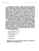
The LM schedule shows the combinations of interest rates and income compatible with equilibrium in the money market. It is the schedule, along which the demand for real money balances. Therefore, since it is:
Real Md = Mp + Mtr (Y) + LP (i)
Equilibrium is when:
Desired demand for real balances = real money supply
Md (Mp, Y, I) = (Ms/P)
Where, Ms is the nominal money supply
Ms is decided by the authority
Ms changes when monetary policy is implemented
Ms/P = real money supply
Real money can change, even if the nominal money supply is fixed, when the general level of price changes. From the equilibrium we derive LM curve:
md (Mp, Y, i) = ms
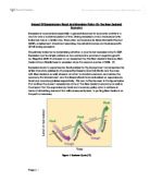
Therefore, LM curve is the locus of these values and it represents the equilibrium ( md = ms) in the money market. The following figure shows how we construct the LM schedule.
DERIVATION LM CURVE
QUADRANT (A) MS QUADRANT (B)
Mtr+Mp (1/V)
M Md=MS
Y1 Y2
Md
QUADRANT (D) QUADRANT (C)
i
r=1 LM
r1
r2 LP
In contrast with the IS schedule, the LM schedule, with a higher income level, it calls for a higher interest rate to obstruct money demand and preserve money market equilibrium with an unchanged money supply. The more a specified increase in income tends to boost the quantity of money demanded, the larger will be the increase in the interest rate required to maintain money market equilibrium and the steeper will be the LM schedule. Correspondingly, the less approachable the quantity of money demanded to a particular rise in interest rates, the larger will be the increase in interest rates required to choke off money demand for a particular increase in income, and the steeper will be the LM schedule. On the other hand, the more the quantity of money demanded responds to interest rates and the less it responds to income, the flatter will be the LM schedule.
We assemble a prearranged LM schedule for a specified supply of real money balances. Presume we now enlarge the supply of real money balances. For a specified income level and a certain height of the money demand schedule in figure (a), the equilibrium interest rate will now be lower in view of the fact that the vertical supply curve has shifted to the right. At apiece income level, a lower interest rate is required to provoke people to hold the additional supply of real balances. Consequently, in figure (b) we must embody an increase in the supply of real money balances as a shift to the right in the LM schedule, showing that the equilibrium interest rate is lower at apiece income level, or, homogeneously, that at apiece interest rate it requires a higher income level to provoke people to hold the additional supply of real balances. On the contrary, a decrease in the real money supply shifts the LM schedule to the left. To diminish the quantity of real balances demanded and maintain money market equilibrium with a lower real money supply, it now takes a higher interest rate at apiece income level.
To go over the main points, we depict an LM schedule for a given real money supply. Moving along the schedule, higher interest rates must go together with higher income to maintain the quantity of real balances demanded in sequence with the permanent supply. Increases in the real money supply, shift the LM schedule to the right. Even though the real money supply can be increased either by an increase in the titular money supply at invariable goods prices or by a drop in goods prices with a given ostensible money supply, we reflect only on the previous device, given that we are still assuming that goods prices are fixed.
Instead of having two separate but interconnected diagrams to point up the markets for goods and money, the IS-LM model allows us to think about both markets in the same diagram. The following figure plots both the IS schedule, showing goods market equilibrium, and the LM schedule, showing money market equilibrium. Only at E are both markets in equilibrium. Hence, the goods and money markets act together to settle on the level of equilibrium interest rate r* and the equilibrium income Y*.
Interest LM
rates
A B
r1
E
r*
r2
D C
IS
Y1 Y* Y2
Income
“Suppose the interest rate is r1. At the income Y1 we would be at the point A on the IS schedule. The combinationr1 and Y1 lead to goods market equilibrium. Nevertheless, at the interest rate r1 it would require an income Y2 for money market equilibrium, at B on the LM schedule. Given the interest rate r1, the income level Y1 is too low for money market equilibrium. With too low an income level, there is not enough money demand to match the given quantity of money supply. With excess supply of money, interest rates will have to be cut to achieve the money supply target. We can repeat this argument until interest rates fall to r*. At that level, aggregate demand and income have risen sufficiently to increase money demand enough to lead to equilibrium in the money market as well as the goods market”. (David Begg, economics, sixth edition, page 419).
ISLM model can be used to examine the effects of fiscal and monetary policy. Assume that the economy is in recession and that the government wishes to raise the level of national income. The three following figures illustrate the policy alternatives.
r LM
r2
r1 IS2
IS1
0 Y1 Y2 Y
The above figure shows the effect of an increase in the government expenditure (G) or a cut in taxes (T), but with no increase in money supply. The IS curve shifts to the right and although income rises to Y2, interest rates rise. The according figure shows the effect of an increase in money supply. The LM curve shifts downwards. Interest rates fall to r3, and this encourages an increase in investment. As a result, income rises to Y3.
r LM1
LM2
r1
r3
IS
0
Y1 Y3 Y
Finally, the following figure shows what happens when the government finances higher government expenditure or lower taxes by increasing the money supply. There is no rise in interest rates and thus, no crowding out. National income rises by a greater amount to Y4.
r LM1 LM2
r1
IS2
IS1
0
Y1 Y4 Y
Drawing a conclusion, the usefulness of fiscal and monetary policy depends on the slope of the two curves. Fiscal policy is more effective when the LM curve is shallow and the IS curve steep. On the contrary, monetary policy is more effective when the LM curve is steep and the IS curve is shallow. Finally, it is arguably acceptable that fiscal and monetary policies will be most effective when applied simultaneously.