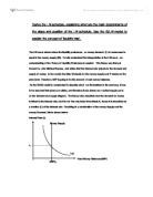
Interest Rate (r)
Money Supply
r1 B
r0 A
L(r,Y1)
L(r,Y0)
Real Money Balances (M/P)
(M/P)0
Above shows what should happen to the interest rate given an increase in the demand for real money balances. Starting at point A, with the equilibrium of (M/P)0, r0, as the economy starts to move into an upturn, the demand for real money balances increases, shifting the L(r,Y) curve from L(r,Y0) to L(r,Y1). As a result of this, causing an increase in the interest rate from r0 to r1, creating a new equilibrium point B.
The above diagram tells us that the demand for real money balances is negatively related to the interest rate. However, there is a positive relationship between the interest rate and an increase in the demand for real money balances. Therefore, by using the increase in the demand for real money balances, it is possible to derive the LM schedule. This is shown below:
Interest Rate (r) Interest Rate (r)
Money Supply
r1 r1
r0 r0
L(r,Y0)
(M/P)
(M/P)0 Y0 Y1
Above is the derivation of the LM schedule, it describes the relationship between the interest rate and Income. When the interest rate is originally at r0, the economy’s money market is in equilibrium, with the money supply equalling the money demand, and as a result shows that the economy should have an income of Y0. Then when incomes are increased to Y1, then as a result increases the demand for money, which consequently, raises the interest rate to r1. It should be noted that the LM schedule cannot be used to calculate the interest rate or income at any given level; it is purely a descriptive device to help explain short-run fluctuations in the financial sector of the economy.
One factor that affects the slope of the LM schedule is the elasticity of the demand for real money balances. For example, is it is very demand inelastic, a very small change in the amount of real money balances held, or demanded, will significantly change the interest rate. The opposite happens when the demand for real money balances is very demand elastic. There would need to be a very significant change in the amount of real money balances demanded in order to change the interest rate.
As it stands, the LM schedule is drawn for a specific money supply curve. Therefore, changes in monetary policy are going to change the money supply curve, which as a result changes the LM schedule. If the government were to increase the money supply, causing a rightward shift in the money supply curve, this will lower the interest rate as the economy slides along the L(r,Y) curve. The LM schedule will shift right as well as a result of this lower interest rate. The opposite happens with a decrease in the money supply. The economy’s interest rate will increase as it slides upwards along the L(r,Y) curve to compensate for the change in the money supply. This will cause the LM schedule to shift left as there is an increase in the interest rate, but no change in income. Below shows the two examples diagrammatically:
Interest Rate (r) Interest Rate (r)
Ms3 Ms1 Ms2 LM3
LM1
LM2
r3
L(r,Y)
(M/P)
(M/P)3 (M/P)1 (M/P)2 Y0
Above shows how differing monetary policies can affect the shifts in the LM curve. LM1 describes the original state of the economy, LM2 describing what happens when the money supply is increased, shown by the shift from Ms1 to Ms2. Whilst LM3 describes what happens when the money supply in decrease, shown by the shift from Ms1 to Ms3.
The LM schedule can help economists explain a situation called the liquidity trap. The liquidity trap is where interest rates are so low, often very close to zero, that people hold their money as cash so they can try to gain in the future, when the interest rate starts to climb upwards. Two famous examples of a liquidity trap are from the Great Depression of the 1930’s and the Japanese economy during the 1990’s.
In diagrammatic terms, the liquidity trap occurs when the elasticity for the demand of real money balances is infinitely zero, which as a result makes the LM curve horizontal as well. Taking the IS/LM model, and adapting the LM curve to represent a liquidity trap, it can become clear as to how difficult it is to get out of a liquidity trap.
Interest Rate (r)
LM1 LM2
r1
IS1
Y1 Y
Taking the original equilibrium or IS1 and LM1, yielding an interest rate of r1 and income Y1. It becomes clear that monetary policy is completely ineffective; this is because tightening monetary policy is impossible as the interest rate is already as low as it can get. Expansionary monetary policy would shift the LM curve outwards, as represented by the shift from LM1 to LM2, however this has no effect on the original equilibrium. In relation to the Japanese case, it was first put forward that they were in a liquidity trap by Paul Krugman, where he also suggested that to get out of the liquidity trap, the government would have to strongly encourage, and almost force consumers to spend rather than hold their cash. Krugman proposed that to do this, the government would have to bring about a period of inflation with the target to be around 4% a year, for a period totalling around 15 years. It was by doing this that Krugman felt would act as a disincentive to save, and cause currency depreciation. This view was quite controversial, as it does make the vital assumption that governments are smart enough to control inflation effectively, and if unsuccessful, could lead to another crisis altogether. This strategy does seem like a good way of escaping the liquidity trap, as by raising the inflation rate above the interest rate, which would create a real loss of on any deposits made in any financial institution. Another way that the crisis was dealt with was by giving customers free shopping vouchers and reforming the tax system to strongly promote consumer spending. Also, since monetary policy was effectively useless, fiscal policy would have to be used to help get out of the trap.
“In November 1998 it instigated additional fiscal measures to stimulate domestic demand. The $195 billion package was the largest ever and included additional spending programmes as well as cuts in personal income tax. Income tax cuts had long been advocated to restore consumer confidence in the economy and to encourage consumer spending and shift the balance between savings and consumption.”
(“Japan In Crisis”, S. Javed Maswood, 2002, pages149-150)
The LM curve shows how consumers behave in the financial markets with respect to their income and the interest rate. Combined with the IS curve, which explains the equilibrium in the goods and services market, is an analytical tool which economists use to explain short run fluctuations in the economy. As shown, it can also help explain the liquidity trap, which was responsible for arguably the two greatest disasters in economic history.
Bibliography
- Mankiw, N.G. (2007), Macroeconomics, (6th Edition), Worth
-
S.Javed Maswood , (2002), “Japan In Crisis”, 1st edition Palgrave