According to the multiplier formula, k=1/(mpw)=1/(1- mpc), the size of the multiplier depends on mpc or on mpw respectively. The marginal propensity to withdraw (mpw) indicates the proportion of a rise in national income that is withdrawn. The marginal propensity to consume (mpc= ΔC / ΔY) indicates the proportion of a rise in national income spent on consumption. The bigger mpc, the smaller is mpw and vice versa since the additional sum of mpc and mpw must be equal to one.
As the mpc gives the slope of the consumption function relating consumption to national income (C= f(Y)), it is flatter in the short run than in the long run.
This is because of the permanent income hypothesis proposed by M. Friedman (1957) that suggests that people base their consumption on what they regard as “normal” income. According to Friedman there are 2 types of income namely transitory and permanent income. Transitory income is temporary income which comes unexpectedly. Permanent income, on the other hand, is the average income that a person expects to receive over a lifetime.
Consumer base their average (permanent) consumption over a long period of time on their average (permanent) income over that period which is a more realistic and with that reasonable approach to consumption as it is then based on long-run/permanent income.
When these consumers experience an unexpected increase in income they are more likely to save most of it than to spend it. This means that transitory income is not the basis of peoples’ consumption. To explain the short- and long-run consumption function we can use these two income-types proposed by Friedman.
The short-run response of an increase in income is only a small change in consumption which is grounded on cautiousness and the uncertainty of the persistence of this increase. As defined earlier this is transitory income which is predominately saved and therefore only slightly enlarges consumption. If the income-increase proves its persistence people will adjust and shift their permanent income expectations up in the long-run. Their living standards will go up as a consequence, i.e. they will spend more money and consumption will increase more. Hence, the mpc is bigger in the long- than in the short-run. The steeper the consumption function and hence the greater mpc (smaller mpw) the bigger will be the rise in Y with an increase in J, i.e. the bigger is the multiplier. Due to the implications of the permanent income hypothesis the consumption function is relatively flat in the short run. When income rises consumption rises only little as much of it is saved. Thus less income will be re-circulated resulting in only a small rise in national income and in a small multiplier. An upward shift in AD then results in the change (d1-c1) in Y and the value of the multiplier is (b1-a1)/(d1-c1).
As the consumption function is, as explained earlier, steeper in the long-run the same upwards shift in the AD schedule results in a bigger change in Y (d2-c2). This can be explained by the fact that as people are able to adjust their consumption patterns to an increase in income they are willing to consume more, therefore more money is re-circulated in the economy which results in a greater rise in national income. Thus the multiplier in the long run (b2-a2)/(d2-c2) is greater than in the short run: (b2-a2)/(d2-c2)>(b1-a1)/(d1-c1).
Theory and diagrams taken from:
D. Begg et al. (2003): Economics 7th edition, McGraw Hill
M. Parkin et al. (2000): Economics 5th edition, Addison Wesley
J. Sloman (2000): Economics 4th edition, Prentice Hall