Correlation and regression

Ibrar Khan AS Use of mathematics coursework

Background information

In statistics, correlation often indicates the strength and direction of a linear relationship between two random variables. If there is no correlation between the two sets of data, the points will be widely scattered and will require a circular shape to enclose them. If the two sets of data have weak positive correlation, the points can be modelled in a broad eclipse sloping upwards from bottom left to top right. Furthermore if the two sets of data have a strong positive correlation, the points lie within a narrow eclipse sloping upwards.

If the two sets of data have weak negative correlation, where one quantity generally increases as the other one decreases, the points can be modelled in a broad eclipse sloping downards from top left to bottom right. If the two sets of data have a strong positive correlation, the points lie within a narrow eclipse sloping downwards.

Finally ‘perfect’ positive correlation (a correlation co-efficient of +1) implies that as one variable moves, either up or down, the other variable will move in lockstep, in the same direction. Alternatively, ‘perfect’ negative correlation means that if one variable moves in either direction the variable that is perfectly negatively correlated will move by an equal amount in the opposite direction, also when all the data points on a scatter diagram accumulate on a straight line we say that they are perfectly positively or negatively correlated.

A correlation coefficient is a number between -1 and +1, which measures the degree to which two variables are linearly related. If there is perfect linear relationship with positive slope between the two variables, we have a correlation coefficient of +1; if there is positive correlation, whenever one variable has a high (low) value, so does the other. If there is a perfect linear relationship with negative slope between the two variables, we have a correlation coefficient of -1; if there is negative correlation, whenever one variable has a high (low) value, the other has a low (high) value. A correlation coefficient of 0 means that there is no linear relationship between the variables.

Lines of best fit can be drawn to determine some useful estimates, but would differ in placement from person to person. Therefore it is useful to have a systematic method that always gives the same result. One procedure commonly used is the “method of least squares”. The equation for the line of best fit according to the method of least squares is ‘y = ax + b’, with gradient ‘a’ and y-intercept ‘b’. A line of best fit determined in this way is called a regression line.

Introduction

I have been provided with results of a year 9 top set mock SAT exam in mathematics. The exam is in three sections, a mental paper, a non-calculator written paper (Paper 1) and a calculator written paper (Paper 2). The top set consists of 65 pupils, 30 male and 35 female. My task is to conduct a study of the results, commenting on any hypothesis and interpreting my views by statistical charts and other terms.

Eliminating any data

A male student, who achieved 29 marks on the non-calculator written paper (Paper 1) and 30 marks on the calculator written paper (Paper 2), did not take the mental test for an unknown reason and therefore I am going to eliminate his data due to incompleteness.

Hypothesis

First of all, I am going to compare the non-calculator written paper (Paper 1) and the calculator written paper (Paper 2) results of the males and females. I predict that ‘on average the male population will have higher marks on the non-calculator written paper (Paper 1) and the calculator written paper (Paper 2) than the female population’. I am going to prove this hypothesis by drawing two ‘Back to back’ Stem and leaf diagrams with one showing the non-calculator written paper (Paper 1) results of both the male and female population and the other showing the calculator written paper (Paper 2) results. A ‘Back to back’ Stem and leaf diagram will facilitate me in finding measures of location such as the median, which is the middle value in an ordered list and the modal value, which is the most common value. Furthermore I am going to find the remaining measure of location, which is the mean. A ‘Back to back’ Stem and leaf diagram cannot assist me in finding the mean as it can with the other measures of location, but the mean can be found by using a simple method, which is dividing the total of values by the number of values. By finding the following measures of location I can compare the non-calculator written paper (Paper 1) and the calculator written paper (Paper 2) results of the males and females and observe which population is the more intelligent in the mathematics top set for year 9.

‘Back to back’ Stem and leaf diagram

Data can be shown in a variety of ways including graphs, charts and tables. A Stem and Leaf Plot is a type of graph that is similar to a histogram but shows more information. The Stem-and-Leaf Plot summarizes the shape of a set of data (the distribution) and provides extra detail regarding individual values. The data is arranged by place value. The digits in the largest place are referred to as the stem and the digits in the smallest place are referred to as the leaf (leaves). The leaves are always displayed to the left of the stem. Stem and Leaf Plots are great organizers for large amounts of information.

Non-calculator written paper (Paper 1)

Male population Female population

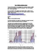
Calculator written paper (Paper 2)

Male population Female population

Stem and leaf diagrams have both advantages and disadvantages in there use. A common advantage would be the fact that you can store a large amount of data in a smaller space, also stem and leaf diagrams can be drawn and filled in more quickly than a line plot. Furthermore it is easy to find the ...

This is a preview of the whole essay

Calculator written paper (Paper 2)

Male population Female population

A common disadvantage in the use of a stem and leaf diagram would be the fact that they can be difficult to read.

Finding the medians using the ‘Back to back’ Stem and leaf diagram

Starting with the non-calculator written paper (Paper 1) for the male population.

0.5 (29 + 1) = 15 th value

Then you start with the highest mark, which for the male population on the non-calculator written paper (Paper 1) was ‘53’ marks and count along, next being ‘49’ and then ‘43’ and so on until you reach the 15 th value, The 15 th value in my case is ‘35’ marks, so therefore, the median mark for the male population on the non-calculator written paper (Paper 1) is 35 marks.

Next, the non-calculator written paper (Paper 1) for the female population.

0.5 (35 + 1) = 18 th value

Then you start with the highest mark, which for the female population on the non-calculator written paper (Paper 1) was ‘49’ marks and count along, next being ‘46’ and then ‘44’ and so on until you reach the 18 th value. The 18 th value in my case is ‘29’ marks, so therefore, the median mark for the female population on the non-calculator written paper (Paper 1) is 29 marks.

After finding the median marks for the non-calculator written paper (Paper 1) of the male and female populations, I can quite honestly articulate that so far my prediction of ‘the male population will have higher marks on the non-calculator written paper (Paper 1) and the calculator written paper (Paper 2) than the female population’ is true and accurate because the median marks for the non-calculator written paper (Paper 1) of the male population was ‘35’ marks, whereas the female population was only ‘29’ marks.

Next, I am going to find the median marks on the calculator written paper (Paper 2) for both the male and female populations by doing a similar process as above.

Starting with the calculator written paper (Paper 2) for the male population.

0.5 (29 + 1) = 15 th value

Then you start with the highest mark, which for the male population on the calculator written paper (Paper 2) was ‘46’ marks and count along, next being ‘45’ and then ‘45’ and so on until you reach the 15 th value. The 15 th value in my case is ‘30’ marks, so therefore, the median mark for the male population on the calculator written paper (Paper 2) is 30 marks.

Next, the calculator written paper (Paper 2) for the female population.

0.5 (35 + 1) = 18 th value

Then you start with the highest mark, which for the female population on the calculator written paper (Paper 2) was ‘51’ marks and count along, next being ‘47’ and then ‘42’ and so on until you reach the 18 th value. The 18 th value in my case is ‘26’ marks, so therefore, the median mark for the female population on the calculator written paper (Paper 2) is 26 marks.

After finding the median marks for the non-calculator written paper (Paper 1) and the calculator written paper (Paper 2) of the male and female populations, I can for definite articulate that my prediction of ‘the male population will have higher marks on the non-calculator written paper (Paper 1) and the calculator written paper (Paper 2) than the female population’ is true and accurate because in the case of ‘median marks’ the male population have higher median marks than the female population in both the non-calculator written paper (Paper 1) and the calculator written paper (Paper 2). On the non-calculator written paper (Paper 1) the male population got ‘6’ marks higher than the female population and on the calculator written paper (Paper 2) the male population got ‘4’ marks higher than the female population.

Finding the modal values using the ‘Back to back’ Stem and leaf diagram

Starting with the non-calculator written paper (Paper 1) for the male population. The mode is defined as the data value that occurs most often. So we are looking for the leaf (number) that occurs the most often on one stem of the diagram. In my case, there are three 5 leafs on the 2 stem (i.e. three data points of value 25), three 5 leafs on the 3 stem (i.e. three data points of value 35) and three 7 leafs on the 3 stem (i.e. three data points of value 37). So the data set is ‘tri-modal’ with modes of 25, 35 and 37. Next, the non-calculator written paper (Paper 1) for the female population, I can see that there are four 9 leafs on the 2 stem (i.e. four data points of value 29), therefore 29 marks is the modal value for the non-calculator written paper (Paper 1) of the female population. Next, I am going to find the modal value of the calculator written paper (Paper 2) for both the male and female populations. Starting with the male population, there are three 7 leafs on the 2 stem (i.e. three data points of value 27), and three 9 leafs on the 2 stem also (i.e. three data points of value 29). So the data set is ‘bi-modal’ with modes of 27 and 29. Finally the calculator written paper (Paper 2) for the female population there are three 3 leafs on the 2 stem (i.e. three data points of value 23), and three 6 leafs on the 2 stem also (i.e. three data points of value 26). So the data set is again ‘bi-modal’ with modes of 23 and 26.

Calculating the mean

Starting with the non-calculator written paper (Paper 1) for the male population.

I add up all the data values from the highest mark, which in my case was ‘53’ to the lowest mark, which is ‘16’ and this should total to 950 marks. Then you divide this number by the number of values, which are 29 males.

950 / 29 = 32.8 marks

It is not possible to get 32.8 marks on an exam so this value can be rounded up to make 33 marks. Therefore the mean of marks on the non-calculator written paper (Paper 1) for the male population was 32.8 or 33.

Next, the non-calculator written paper (Paper 1) for the female population.

I again add up all the data values from the highest mark, which in my case was ‘49’ to the lowest mark, which is ‘16’ and this should total to 1078 marks. Then you divide this number by the number of values, which are 35 females.

1078 / 35 = 30.8 marks

It is not possible to get 30.8 marks on an exam so this value can be rounded up to make 31 marks. Therefore the mean of marks on the non-calculator written paper (Paper 1) for the female population was 30.8 or 31.

After finding the mean of marks for the non-calculator written paper (Paper 1) of the male and female populations, I can quite honestly articulate that again my prediction of ‘on average the male population will have higher marks on the non-calculator written paper (Paper 1) and the calculator written paper (Paper 2) than the female population’ is true and accurate because the mean marks for the non-calculator written paper (Paper 1) of the male population was ’32.8’ or ‘33’ marks, whereas the female population was only ’30.8’ or ‘31’ marks.

Next, I am going to find the mean marks on the calculator written paper (Paper 2) for both the male and female populations.

Starting with the calculator written paper (Paper 2) for the male population.

I add up all the data values from the highest mark, which in my case was ‘46’ to the lowest mark, which is ‘20’ and this should total to 920 marks. Then you divide this number by the number of values, which are 29 males.

920 / 29 = 31.7 marks

It is not possible to get 31.7 marks on an exam so this value can be rounded up to make 32 marks. Therefore the mean of marks on the calculator written paper (Paper 2) for the male population was 31.7 or 32.

Next, the calculator written paper (Paper 2) for the female population.

I again add up all the data values from the highest mark, which in my case was ‘51’ to the lowest mark, which is ‘14’ and this should total to 1015 marks. Then you divide this number by the number of values, which are 35 females.

1015 / 35 = 29 marks

Therefore the mean of marks on the calculator written paper (Paper 2) for the female population was 29.

After finding the mean marks for the non-calculator written paper (Paper 1) and the calculator written paper (Paper 2) of the male and female populations, I can again for definite articulate that my prediction of ‘the male population will have higher marks on the non-calculator written paper (Paper 1) and the calculator written paper (Paper 2) than the female population’ is true and accurate because in the case of ‘mean marks’ the male population have higher mean marks than the female population in both the non-calculator written paper (Paper 1) and the calculator written paper (Paper 2). In the case of mean, on the non-calculator written paper (Paper 1) the male population got on average ‘2’ marks higher than the female population and on the calculator written paper (Paper 2) the male population got on average ‘3’ marks higher than the female population.

In summary I can quite truthfully say that my hypothesis that ‘on average the male population will have higher marks on the non-calculator written paper (Paper 1) and the calculator written paper (Paper 2) than the female population’ was true and accurate. I used a ‘Back to back’ Stem and leaf diagram to assist me in finding measures of location such as the median and the modal value. I also found the mean, which gave me an average of the marks for each population on a certain exam, all this facilitating me in trying to prove my hypothesis correct.

Hypothesis

For my new hypothesis I am primarily going to investigate the correlation between the mental test and the non-calculator written paper (Paper 1) of the male and female populations. At first I will create a scatter diagram in Microsoft excel, with the mental test marks of the male and female populations on the y-axis and the non-calculator written paper (Paper 1) marks on the x-axis. I predict that ‘there will be a weak positive correlation between the mental test and the non-calculator written paper (Paper 1) of the male and female populations, the points on the scatter diagram will be modelled in a broad eclipse sloping upwards from bottom left to top right. Furthermore I predict the value of the correlation coefficient to be between 0 < r ≤ 0.5, which would indicate a weak positive correlation’. I will be able to find the value of the correlation coefficient by using a CASIO graphical calculator (CFX-9850GC PLUS). Next on my scatter diagram I will mark the mean point and draw a line of best fit, which will go through the mean point. By doing the above I will be able to prove whether my hypothesis (prediction) is precise or not.

After using Microsoft excel to draw my scatter diagram and observing the correlation, I can quite truthfully articulate that my hypothesis ‘there will be a weak positive correlation between the mental test and the non-calculator written paper (Paper 1) of the male and female populations, the points on the scatter diagram will be modelled in a broad eclipse sloping upwards from bottom left to top right. Furthermore I predict the value of the correlation coefficient to be between 0 < r ≤ 0.5, which would indicate a weak positive correlation’ is incorrect and erroneous because the value of the correlation coefficient that I acquired after using a CASIO graphical calculator (CFX-9850GC PLUS) was ‘r = 0.705’, which indicates a strong positive correlation and the points lie within a narrow eclipse sloping upwards. I have also marked the mean point on my scatter diagram and drawn a line of best fit as I said I would accomplish in my hypothesis.

Next, on a new copy of the equivalent scatter diagram I am going to draw a regression line, in the form of ‘y = ax + b’, with gradient ‘a’ and y-intercept ‘b’. The values of the gradient ‘a’ and the y-intercept ‘b’ can be found with the use of a CASIO graphical calculator (CFX-9850GC PLUS). The way to do this on a CASIO graphical calculator (CFX-9850GC PLUS) is from the main menu you go to ‘list’ and press execute. Enter the data into ‘list 1’ and ‘list 2’ and then press ‘menu’, which will take you back to the main menu screen. Then go to ‘stat’ and press execute, the same lists of values you just entered should appear. After that you press ‘F2’ just below ‘calc’ on the screen, then press ‘F3’ just below ‘REG’ on the screen and finally press ‘F1’ just below ‘X’ on the screen. This will provide you with values of the gradient ‘a’ and the y-intercept ‘b’. After I have found the values of the gradient ‘a’ and the y-intercept ‘b’ I will substitute them into the equation ‘y = ax + b’ and draw the regression line. Using a CASIO graphical calculator (CFX-9850GC PLUS) is one way of finding the parameters, which would then be substituted into the equation ‘y = ax + b’ but I know of an alternate way, which would be even simpler to use. On a new copy of the equivalent scatter diagram in Microsoft excel you click on the ‘Chart’ icon and a drop down list emerges, select ‘Add trendline’ and a dialogue box appears. Select the ‘linear trend/regression type’. Then you choose the ‘Options’ tab and if you desire for the equation to display on the scatter diagram along with the regression line then select ‘Display equation on chart’ and click OK to close the dialogue box. This will display an accurate regression line on the scatter diagram along with the equation in the form of ‘y = ax + b’. I am going to use this method instead of the CASIO graphical calculator (CFX-9850GC PLUS) because I believe it is more straightforward.

After using Microsoft excel to draw the regression line on a new copy of the equivalent scatter diagram, I have found the equation of it to be ‘y = 0.3872x + 6.2063’. This equation in the form of ‘y = ax + b’ was simply found by exploiting what I explained above.

Now that I have found the equation of the regression line, which is ‘y = 0.3872x + 6.2063’, I can use the equation or the regression line to estimate the absent mental test mark of the male student. I know that the student scored 29 marks on the non-calculator written paper (Paper 1) and therefore I substitute ‘29’ into the equation in place of ‘x’. This will modify the equation to:

y = (0.3872 x 29) + 6.2063

= 17.4 marks

It is not possible to get 17.4 marks on an exam so this value can be rounded down to make 17 marks. By using the equation of the regression line I have estimated the absent mental test mark of the male student to be 17 marks.

Hypothesis

For my new hypothesis I am going to investigate the correlation between the mental test and the calculator written paper (Paper 2) of the male and female populations. At first I will create a scatter diagram in Microsoft excel, with the mental test marks of the male and female populations on the y-axis and the calculator written paper (Paper 2) marks on the x-axis. I predict that ‘there will be a strong positive correlation between the mental test and the calculator written paper (Paper 2) of the male and female populations, the points on the scatter diagram will lie within a narrow eclipse sloping downwards. Furthermore I predict the value of the correlation coefficient to be between 0.5 < r ≤ 1, which would indicate a strong positive correlation’. I will be able to find the value of the correlation coefficient by using a CASIO graphical calculator (CFX-9850GC PLUS). Next on my scatter diagram I will mark the mean point and draw a line of best fit, which will go through the mean point. By doing the above I will be able to prove whether my hypothesis (prediction) is precise or not.

After using Microsoft excel to draw my scatter diagram and observing the correlation, I can quite truthfully articulate that my hypothesis ‘there will be a strong positive correlation between the mental test and the calculator written paper (Paper 2) of the male and female populations, the points on the scatter diagram will lie within a narrow eclipse sloping downwards. Furthermore I predict the value of the correlation coefficient to be between 0.5 < r ≤ 1, which would indicate a strong positive correlation’ was true and accurate because the value of the correlation coefficient that I acquired after using a CASIO graphical calculator (CFX-9850GC PLUS) was ‘r = 0.679’, which indicates a strong positive correlation and the points lie within a narrow eclipse sloping upwards as I expected. I have also marked the mean point on my scatter diagram and drawn a line of best fit as I said I would accomplish in my hypothesis.

Next, on a new copy of the equivalent scatter diagram I am going to draw a regression line, in the form of ‘y = ax + b’, with gradient ‘a’ and y-intercept ‘b’. The values of the gradient ‘a’ and the y-intercept ‘b’ can be found by using Microsoft excel and following the procedure I typed above for the previous hypothesis. After using Microsoft excel to draw the regression line on a new copy of the equivalent scatter diagram, I found the equation of it to be ‘y = 0.3809x + 6.9837’.

Now that I have found the equation of the regression line, which is ‘y = 0.3809x + 6.9837’, I can use the equation or the regression line to again estimate the absent mental test mark of the male student. I know that the student scored 30 marks on the calculator written paper (Paper 2) and therefore I substitute ‘30’ into the equation in place of ‘x’. This will modify the equation to:

y = (0.3809 x 30) + 6.9837

= 18.4 marks

It is not possible to get 18.4 marks on an exam so this value can be rounded down to make 18 marks. By using the equation of the regression line I have estimated the absent mental test mark of the male student to be 18 marks.

Reflecting upon the past two hypothesis I can enunciate that the correlation between the mental test and the non-calculator written paper (Paper 1) of the male and female population is stronger than the correlation between the mental test and the calculator written paper (Paper 2) because the correlation coefficient for the mental test and the non-calculator written paper (Paper 1) of the male and female population was ‘r = 0.705’, whereas the correlation coefficient for the mental test and the calculator written paper (Paper 2) was ‘r = 0.679’. As I have explained in the background information the more near to ‘1’ the value of ‘r’ is the stronger the correlation between the two variables. Furthermore by drawing the regression lines on the scatter diagrams and finding the equation of the regression lines in the form of ‘y = ax + b’, with gradient ‘a’ and y-intercept ‘b’, I have been able to estimate the absent mental test mark of the male student. The scatter diagram showing the correlation between the mental test and the non-calculator written paper (Paper 1) of the male and female population had ‘y = 0.3872x + 6.2063’ as the equation of the regression line and gave an estimate mental test mark of 17. In contrast to the scatter diagram showing the correlation between the mental test and the calculator written paper (Paper 1), which had

‘y = 0.3809x + 6.9837’ as the equation of the regression line and gave an estimate mental test mark of 18. From the two estimated mental test marks of the male student that I acquired, I consider the estimated ’17 marks’ to be more accurate than the estimated ’18 marks’ because the correlation is stronger between the mental test and the non-calculator written paper (Paper 1) of the male and female population with a correlation coefficient of ‘r = 0.705’, compared the mental test and the calculator written paper (Paper 2) which had a correlation coefficient of ‘r = 0.679’.

Hypothesis

For my new hypothesis I am going to compare the correlation coefficients of the male and female population in terms of the mental test and the non-calculator written paper (Paper 1) results. I predict that ‘the correlation coefficient for the male population will be larger than the correlation coefficient for the female population. Furthermore I predict the values of the correlation coefficients for both the male and female population to be between 0.5 < r ≤ 1, which would indicate strong positive correlations’. I will be able to find the values of the correlation coefficients by using a CASIO graphical calculator (CFX-9850GC PLUS).

The method to find the correlation coefficient using a CASIO graphical calculator

(CFX-9850GC PLUS) is from the main menu screen you go to ‘list’ and press execute. Enter the data into ‘list 1’ and ‘list 2’ and then press ‘menu’, which will take you back to the main menu screen. Then go to ‘stat’ and press execute, the same lists of values you just entered should appear. After that you press ‘F2’ just below ‘calc’ on the screen, then press ‘F3’ just below ‘REG’ on the screen and finally press ‘F1’ just below ‘X’ on the screen. This will provide you with the value of the correlation coefficient (r) for the set of data. After carrying out the method above I found the correlation coefficient of the mental test and the non-calculator written paper (Paper 1) for the male population to be ‘r = 0.743’ and the correlation coefficient for the female population to be

‘r = 0.704’. Now that I have found the correlation coefficients of the mental test and the

non-calculator written paper (Paper 1) for the male and female populations I can quite truthfully articulate that my hypothesis ‘the correlation coefficient for the male population will be larger than the correlation coefficient for the female population. Furthermore I predict the values of the correlation coefficients for both the male and female population to be between 0.5 < r ≤ 1, which would indicate strong positive correlations’ was true and accurate because the correlation coefficient for the male population, which was ‘r = 0.743’ was larger than the correlation coefficient for the female population, which was ‘r = 0.704’. Furthermore both correlation coefficients that I acquired are in the region of 0.5 < r ≤ 1, which would indicate strong positive correlations.

Hypothesis

For my new hypothesis I am going to compare the correlation coefficients of the male and female population in terms of the mental test and the calculator written paper (Paper 2) results. On this occasion I predict that ‘the correlation coefficient for the female population will be larger than the correlation coefficient for the male population. Furthermore I again predict the values of the correlation coefficients for both the male and female population to be between 0.5 < r ≤ 1, which would indicate strong positive correlations’. I will be able to find the values of the correlation coefficients by using a CASIO graphical calculator (CFX-9850GC PLUS).

After carrying out the method I explained in the previous hypothesis I found the correlation coefficient of the mental test and the calculator written paper (Paper 2) for the male population to be ‘r = 0.775’ and the correlation coefficient for the female population to be ‘r = 0.698’. Now that I have found the correlation coefficients of the mental test and the calculator written paper

(Paper 2) for the male and female populations I can quite truthfully articulate that my hypothesis ‘the correlation coefficient for the female population will be larger than the correlation coefficient for the male population. Furthermore I again predict the values of the correlation coefficients for both the male and female population to be between 0.5 < r ≤ 1, which would indicate strong positive correlations’ was incorrect and erroneous because the correlation coefficient for the male population, which was ‘r = 0.775’ was larger than the correlation coefficient for the female population, which was ‘r = 0.698’. A fraction of my hypothesis that was proved correct was both correlation coefficients that I acquired were in the region of 0.5 < r ≤ 1, which would indicate strong positive correlations.