Handling the Data
I also examined accuracy of the data, as I can verify the truthfulness of my data I will examine it on face value, I have ignored any data that falls outside of 2 decimal places, weights that are not within the parameters 30-100kg and heights outside 1-2 metres. I have decided to eliminate these values as I consider them to be abnormal and biased, I can conclude this by examining BMI, as I am aware that any-one with a body mass Index lower than 18 or higher than 35 is not typical. This applies for height as upon examining heights of my class mates it is apparent that standard height is not blow 1m or above 2m.
Obtaining evidence for analysis
My analysis will concern the differentiation of boys against girls, as I am aware, from the age of 11 it is apparent both genders take on a from of change and depending on their personal chemistry a change in weight and height is one of the major factors within adolescence.
By obtaining data that I can tabulate I can carry out a series of comparisons and conclude conclusions concerning my applied data.
There are a range of statistical calculations I can make use of.
I am aware I can obtain the following, for both genders and both height and weight:
- Frequency distribution
- Mean;
- Mean deviation;
- Standard deviation;
- Median;
- Range;
- Inter-quartile range;
- Central tendency;
- Measure of dispersion or spread;
- Distribution.
Mode = Value that occurs most in a data set. Not a very useful measure of central tendency.
Median = Middle value from a set of ranked observations. Useful for highlighting the typical value of a data set.
Mean = Sum of a set of observations divided by the number of observations in a data set, most widely used measure of central tendency. Also can be calculated as a weighted mean for grouped data
Standard Deviation = Measures or depicts the amount of spread or variability in a data set; how typical of a whole distribution the mean actually is. It is apparent, the larger the Standard Deviation, the greater the spread of observations and the less typical the mean.
Standard Deviation or Variance to compare locations or regions is an absolute measure.
Mean = A measure of central tendency calculated by dividing the sum of the scores in a distribution by the number of scores in the distribution. This value best reflects the typical score of a data set when there are few outliers and/or the dataset is generally symmetrical.
Box plot = Summary plot based on the median, quartiles, and extreme values. The box represents the inter-quartile range which contains the 50% of values. The whiskers represent the range; they extend from the box to the highest and lowest values, excluding outliers. A line across the box indicates the median.
Skewness = Measures the degree to which data values are evenly or unevenly distributed on either side of the mean. If a majority of the values in a data set fall below the mean, then data are positively skewed with the tail of the histogram falling to the right. If a majority of the values fall above the mean, then data are negatively skewed and the tail of the histogram will fall to the left.
As I have limited amount of time given for this investigation I will consider the importance of the above actions before I carry any of them out.
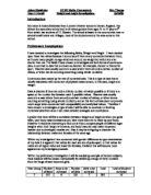
Histogram to compare the Heights for boys and girls
Histogram = Graphic representation of grouped data along two axes
I have chosen to draw a histogram of the heights of the boys and girls within my sample. This will require the grouping of both boys and girls as so I can accumulate frequency and frequency density. Class widths need to be appropriate as so their individual frequency are of tabulating range, as so I can conclude a clear distribution.
I have created a table below which displays the frequency distribution and frequency density for my samples.
Frequency = frequency density x class width interval
Boy’s heights (m)
Girl’s heights (m)
Boy’s weights (kg)
Girl’s weights (kg)
The above sets of data were utilised within figure 1.1, which concerns each genders heights. I have plotted my Histograms as so boys and girls exist within the same graph as so I can make direct comparisons. A histogram allows me to assimilate distribution of the concerned information more quickly than if I were to simply examine the above tables, a graph demonstrates the information clearly and conclusions such as, for example a lack in symmetry, or skew can be concluded.
What is the mean and deviation?
I wish to calculate the means and standard deviations using raw data as so I can obtain additional statistics for my comparison.
I used my calculator to obtain the mean and standard deviation for both genders, using my data for heights and then weights.
Height
Weight
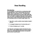
Cumulative curves of weights of both genders
Within the above tables concerning frequency and frequency density for both boys and girls weights I have also calculated the cumulative frequency as so I could create a histogram of these results (figure 1.2)
I can use my graph to analyse the relationship between the data for boys and girls. These two cumulative corves will be plotted within the same graph as so I can carry out a better analysis
Median weight (kg):
Boys = 55
Girls = 48.5
I was able to obtain the median values for each sex easily as my results from my sample were put into a table within a spreadsheet and so I was able to arrange the data in ascending weight order and pinpoint the middle value.
Once the data is arranged in order of ascending height, I can conclude:
Weight range (kg):
Boys = 35-93
Girls = 33-72
Attaining Lower, Upper and inter-quartile range
I was able to obtain these results by pinpointing the intervals 25 percentile, 50 percentile and 75 percentile on my graph and reading off the corresponding data, this was simplified by the fact that weight is a continuous variable, it is a continuous approximation of the distribution of values.
Scatter diagrams of weight against height for boys and girls
This graph enables me to look at any possible correlation between the two variables, height and weight. I can deuce the coefficient, depending on the degree of correlation with line of best fit and plotted points. (Figure 1.3)
Summary of findings from preliminary investigation
My results lead me to believe that in general terms that the central tendency for boys heights is within the range 1.60-1.65 metres and girls, both ranges 1.60-1.65 and 1.70-1.75 metres. I can conclude from the standard deviation for boys concerning both weight and height, suggests that the boy’s values vary more than the girls thus meaning their mean is less typical. It appears that in fact the girls vary less concerning height. Interestingly the boys and girls mean height is the same and their mean weights do not vary too greatly.
These values indicate that a typical weight for boys within Lytchett Minster School, aged from 11-16 is greater than for girls within the same parameters.
As observed by the product of standard deviation, boys are more spread out and have a wider range compared to girls.
These results indicate, in general that both sexes follow a trend concerning weight until their weights until they reach 50 kg. Evidence suggests that 15% of boys are above 68kg, and 15% girls are above 57kg a difference of 11kg. I can also conclude that 50% of boys are above the median weight of 55kg and 73% of girls are above the median weight of 48.5kg. The plotted points on my scatter graphs for both sexes demonstrating weight dependant on height. Both sexes demonstrated a lack of correlation and the deviation from the line of best fit illustrates a wide spread, especially concerning boys.
Analysis
Using my provisional conclusions, I have collected some issues I feel need further investigation. My Histogram indicated that both sexes follow a trend in increasing height until their weight exceed around 50kg, therefore there could be a point where boys weights and heights exceed girls, or that girls start to grow in weight at a more proportional weight to each other and reach a steady weight before boys.
My original approach to sampling of pupils involved a Quota sampling of 5% from each sex and 10% of the whole school.
I would like to take a more detailed look at the school, this time exceeding the percentage by a further 10% so an over all school sample of 20%.
Considering my proposed hypothesis I am going to conduct a survey across year groups rather than the school as a whole, as I do not believe a further look at the generalised patterns of height and weight for boys and girls will help my theory any further than before.
I am going to examine year groups 7 and 11 as so I can pinpoint whether in fact:
- Girls appear to mature at a steadier rate than boys after a certain point, and finish their growth spurt before boys reach their full potential.
I have chosen these two year groups as a comparison as they are at each end of my available age range and I believe will produce the most promising results.
Depending at the outcome of this search I will consider whether it is necessary for me to take a further look at year groups in more detail.
To ensure my testing is fare and candidates have an equal chance of being picked I have decided to use stratified random sampling dividing up the school into years and genders. This is basically finding the ratio of the total number of values you want from each group.
A Sample of 50% sample of each boys and girls from the combined year groups 7 and 11 which have 282 and 170 pupils
Total number of pupils = 170+282= 452
Within this I wish to take a sample of 10% sample in total.
Therefore the following calculations correspond to my sample:
Number of boys from year 7 = 151/452 x 120=40
Number of girls from year 7 = 131/452 x 120=35
Number of boys from year 11= 84/452 x 120=22
Number of girls from year 11 = 86/452 x 120= 23
This then is used to find 40 random pupils from year 7 boys, 35 random pupils from year7 girls and so on.
Year 7 Boys Heights and Weights:
Year 7 girls Weights and Heights:
Year 11 Boys Weights and Heights:
Year 11 Girls Weights and Heights:
Median weight (kg):
Year 7 Boys = 46
Year 7 Girls = 38
Year 11 Boys = 56
Year 11 Girls =48
Year 7 Height
Year 7 Weight
Year 11 Height
Year 11 Weight
The below Graphs are not to the same height scale, this was because the results were either to close together and hard to see the separate results, or spread out over a range of height.
The above scatter diagrams Indicate to me what to expect when I compile my scatter diagrams in more detail.
Equation for line of best fit
y = mx + c (m = gradient and c = y intercept).
To find the equation for the line of best fit on any graph you need to find the gradient of the line and the y intercept. So you can substitute them into the equation for every line which is y = mx + c. So therefore I need to find them for my graphs.
For example if the gradient on my graph was 40, I could substitute this into my equation: y = 40x + c
Now because my line doesn’t go through the y-axis we have to work out where about it would normally go so I need to substitute in 2 values off my graph. I have chosen them as:
x = 1.4
y = 42
So I need to replace x and y to find c:
42 = 40 x 1.4 + c
42 = 56 + c ...
Calculating correlation coefficients
To make accurate comparisons of the two sets of data for each sex and age, I will use spearmans rank. Spearmans rank will show me how closely related height is to weight. Because I have to do the ranking four times, I have decided to only use a sub-sample of ten random people from years 7 and 11 for boys and girls. I will choose the people for my sample via a random number generator on my calculator however, my calculator goes into the second decimal place so I will round up to the nearest whole number. After I have worked out the difference between the ranks squared (d²) I will then use the following equation to calculate the correlation coefficient:
1-6Σd² / n(n²-1)
Year 7 boys
The sum of d² is 71.5
1 – 6 x 71.5/10(10²-1) = 0.56
Year 7 Girls
The sum of d² is 93.50
1 – 6 x 93.50/10(10²-1) = 0.43
Year 11 Boys
The sum of d² is 5.50
1 – 6 x 5.50/10(10²-1) = 0.96
Year 11 Girls
The sum of d² is 117
1 – 6 x 117/10(10²-1) = 0.29
Conclusions
I can tell from these scatter graphs first of all that the girls have a poorer correlation than the boys, this is also proved by my spearmans ranking where I discovered that the correlation coefficient is much greater for boys than for girls. Although the boys have better correlation, the girls have a closer height bracket whereas the boys have a bigger height bracket and a better correlation. In both of the graphs the majority of people are in the 1.6m to 1.8m range. The boys height however continues after 1.8m unlike the girls.
Very like in year 7 the girls weight is not spread out and the majority are still compacted into the 40kg to 60 kg weight range, although it is now more spread out because before it was all nearly on the 40kg line whereas now it is more spread out but still very compact. The boy’s weight is spread out mainly in the 40kg to 80kg range. This shows us that while the girls are fairly uniform in weight the boys are a lot more varied. Like my first prediction the boys are heavier then the girls by year 11.
I can tell from the year 11 cumulative frequency graph for weight that the boys are heavier because the graph ends later for boys then the girls. Also the boys have a greater inter-quartile range. I can tell this because of the shape of the curves. The girls have a tight distribution. I can also tell from the year 11 cumulative frequency graph for height that boys are taller since because many more boys are still on the graph even after the tallest girl has been counted for.
Evaluation
I think that my investigation has been a complete success in proving my original hypothesis, however I do think that I should have made my original samples a little larger, also I think that my sub-sample for spearmans rank was too small as the correlation would have greatly varied if one result was different as there was such a small number of samples. Apart from that I think I have proved that females tend to be of the same weight, but with varied heights, making them have poor correlation, and men tend to be spread over a wide range of heights and weights, but have both strongly related.