Below is all of the data I will be sampling:
Another method of sampling is random sampling. This can be used to obtain a set of 25 different cars to analyse. This is very bias because every car would be given a number using a random number generator. This would make the data bias because an anomaly car would have been included and may have possibly been included many times over therefore making the data unreliable.
Hypothesis
My first prediction is that when mileage increases, the percentage decrease of the price will also increase. This is because people will assume that if the car has been driven more then its performance will not be as high and people will not want to pay as much for the car. Also, because both values increase I believe that a graph showing % decrease of price against mileage would show positive correlation.
Below I have predicted how this graph may look.
Before I can investigate my first hypothesis I will need to work out the price percentage decrease for each car I am sampling. In order to do this I will need to use the formula Decrease in price/starting price x 100.
I will now do a scatter graph for this hypothesis.
The first thing that I spotted was that the scatter graph contained positive correlation. This means that my prediction was correct because as the cars’ mileage’s increased the percentage decrease of second hand prices also increased, thus meaning the more a car had been used by it’s previous owner the cheaper it became.
A line of best fit was also worked out in order to help me work out whether there were any anomalies of which I feel there were none. Also now that a line of best fit has been worked out I can use excel to find out the correlation coefficient. This has a scale from –1 (showing negative correlation) to 1 (showing positive correlation). The graph above has a correlation coefficient of 0.6026.This means that the graph shows positive correlation.
Also, using excel I can work out the equation for the line on the graph. To do this I will need to use the formula y=mx+c (m is the gradient of the line and c is the intercept).
For the graph above the equation of the line is .y=0.0007x + 32.42.
Conclusion
From investigating this hypothesis I have found out that mileage is definitely a variable which affects the second hand price of a car. However there still may be other variables which affect the second hand price of a car. I will now attempt to investigate these other variables.
Hypothesis
I believe that another variable which will affect the second hand price of the car, is the age of the car. I predict that the older the car is the cheaper it is. There are two reasons for this:
- The older a car is, it is likely that it has been used more and has a greater mileage.
- The older a car becomes, the less aesthetically pleasing it looks compared to newer models of cars on the market and so people will be less willing to pay much for an older car.
Also as both of these values increase I think there will be positive correlation shown in the scatter graph: % depreciation against age. Below I have made a prediction graph representing how I think the graph for this hypothesis will look.
Below is the scatter graph showing Percentage decrease of Price against the age of the cars:
Again the first thing I spotted was that the graph showed positive correlation.
This proved my prediction correct because it meant that as the age of the car increased, so did the percentage decrease of its second hand price, thus meaning the older a car is the cheaper it will be.
The correlation coefficient for this graph is 0.7052. This also proves that the above graph contains positive correlation.
The equation for the line of best fit in this graph is y=6.7323x + 28.349.
There were also no anomalies.
Conclusion
From investigating this hypothesis I have found that the age of a car is also a variable which affects the second hand price of a car.
From the data given to me I now believe that the age of a car and its mileage are the two key variables which affect the second hand price of a car. I do not think that any other variables will show correlation because variables such as the brand of a car and engine size are chosen due to the personal liking of the customer purchasing the car. However in order to be sure I shall investigate the percentage decrease of second hand price against the engine size of a car.
Correlation coefficient = 0.0004 (this means that there isn’t really any correlation shown in this graph).
The first thing I spotted here, is that the graph shows no correlation. This proved my prediction correct. This is because different customers will be purchasing cars for different reasons e.g. a more experienced driver would probably prefer a car with a larger engine where as an inexperienced driver would prefer a smaller engine in order to keep car insurance costs down etc. Therefore different customers will choose the car which most suits their needs, thus not affecting the second hand price of a car.
Final Conclusion
Finally, I have come to the conclusion that the two variables which most affect the second hand price of a car are:
-
Mileage- this is because people will assume that if a car has been driven more, then its performance will decrease and people will not be willing to pay as much for this car.
-
Age- the older a car is, the likelier that it has been used more and has a greater mileage. Also the older a car becomes, the less aesthetically pleasing it looks compared to newer models of cars on the market and so people will be less willing to pay much for an older car.