From this frequency polygon, it is clear that there are more boys who weigh more than the girls, and that it seems the boys have a wider range of weights.
From this frequency polygon, we can see that there is a wider range for the girls than there is for the boys.
Estimated Mean, median interval, mode and range.
BOYS
40 2120
Estimated mean = 2120 ÷ 40 = 53 estimated mean = 53
Median Interval
To find the median, we need to find the Cumulative frequency.
The median is the middle value. I have 40 samples, therefore,
40/2 = 20. Therefore I need to look at the cumulative frequency to find the 20th term. I can see from the table that the median interval lies between 50 < w ≤60.
Mode
The mode is the most common term (highest frequency).
The modal interval for boys’ weight is 51 < w ≤60.
Range
To get the range, you minus the lowest term from the highest term.
Therefore; 86 – 35 = 51
GIRLS
40 1960
Estimated mean =1960 ÷ 40 = 49 estimate mean = 49
The average mean for the weight of girls is lower than the average weight of boys, which proves that boys have generally a higher weight than girls.
Median interval
40 = 20
2
I can see from the table that the median interval lies between 41 < w ≤ 50.
Mode
The most frequent weight lies between 41 < w ≤50.
Range
72 – 30 = 42
Boys
40 725
Estimated Mean =725 ÷ 40 = 19 estimate mean = 18.125
Median interval
40 + 1 = 20.5
2
I can see from the table that the median interval lies between 16< h ≤ 20
Mode
The mode is the most common term (highest frequency). In this case, the mode is 16< h ≤ 20 because that has the highest frequency.
Range
40 – 3 = 37
GIRLS
40 745
745 ÷ 40 = 18.625 estimated mean
The girls estimated mean is slightly higher then the boys estimated mean (by .5), which shows girls watch slightly more then TV then the boys.
Median
40 + 1 = 20.5
2
The median interval in this case lies between 16< h ≤ 20.
The boys and girls have the same median interval that suggests both boys and girls watch similar amounts of television.
Mode
The mode is the term, which has the highest frequency. In this case, the mode is 11< h ≤ 15.
Range
40 – 3 = 37
Stem and leaf
Since the data is grouped into class intervals, it also makes sense to record it in a stem and leaf diagram. This will make it easier to read off the median values.
Boys’ weight
A stem and leaf diagram can be used to work out the median. In this case there are twenty numbers up to and including 53, and twenty numbers at 54 or above therefore the median is:
53 +54 = 107 = 53.5
2 2
Girls’ weight
In this case there are twenty numbers up to and including 48, and twenty numbers at 49 or above therefore the median is:
48 + 49 = 97 = 48.5
2 2
Hours of television watched by boys a week
In this case, there are twenty numbers up to and including 17, and twenty numbers at 17 or above therefore the median is:
17 +17 = 34 = 17
2 2
Hours of television watched by girls a week
In this case, there are twenty numbers up to and including 17, and twenty numbers at 18 or above therefore the median is:
17 + 18 = 35 = 17.5
2 2
From these Stem and Leaf diagrams I can see that boys weigh more as their median was 5Kg higher and that girls watch slightly more TV as their median was .5 of an hour higher. This information agrees with the information I gathered from my estimated means above.
Scatter diagrams
Now I will use scatter diagrams. I will make a scatter diagram and I will observe the correlation of weight against hours of T.V watched a week. The correlation will show me what affect each factor has on each other. I would expect that the weight of a child would be higher with the more hours of T.V they watch. I would predict this because I would logically think that the child who watches more T.V would do less exercise and would have a higher weight because they would be sitting in front of a television instead of being active. Scatter diagrams is a very important part of my coursework.
The results I have gathered from these scatter graphs are very strange and I did not expect this type of result. The weak negative correlation of the line of best fit suggests that the less T.V the girls and boys of Mayfield High watch, the more they weigh. I would have expected that the children who watch more T.V will weigh more, but this is not the case in Mayfield High. Maybe all the children who watch a lot of T.V do exercise whilst watching T.V, or maybe the random sample I picked by chance favoured students who were naturally thin. This is not what I would have expected.
I will now look further into the correlation between hours of TV watched and weights by using a technique called spearmen’s rank to see more clearly the strength of the correlations, wherever negative or positive, spearman’s rank provides us with a number between 1 and –1, 1 being a perfect positive correlation and –1 being a perfect negative correlation.
I can see from spearman’s rank that there is a very weak negative correlation with boys and girls that agrees with my scatter graphs, this more clearly shows how weak the correlation is, it seems to be so small that there is barely any correlation at all, the correlations being –0.11 for boys and –0.15 for girls. 0 means complete randomness so my result is quite close to this meaning weight and watching TV are possibly unrelated completely and I that definitely the more TV watched does not mean the heavier you are, in fact from spearman’s graph I could only say that the more TV watched the thinner you are, but I believe that since the number is so close to 0, there is not any real link between weight and the amount of TV watched.
Cumulative Frequency curves
The best way of representing this data on a diagram is to draw cumulative frequency curves. If the curves are drawn on the same axis it is easier to compare the results.
When plotting cumulative frequency graphs, we plot the end point of the interval on the horizontal axis, against the cumulative frequency on the vertical axis.
Cumulative frequency can be a very powerful tool when comparing different sets of data.
Average no. Hrs of T.V watched a week
The following tables show the cumulative frequency for average number of hours of T.V watched a week, boys and girls.
Boys
Girls
Now I will draw my Graph:
Weight
I will now do a cumulative frequency table for the boys’ and girls’ weight.
Boys
Girls
Now I will draw my Graph:
From these cumulative frequency graphs I have learnt regarding hours of TV watched that girls watch more, as their median is higher by 1 hour and upper quartile is a lot higher by 6 hours, but girls also have a much larger inter quartile range showing there are some girls who don’t watch that much but some who watch a lot. I also learnt regarding weight that boys weigh clearly more as their median is 4.5kg higher and both upper and lower quartiles are higher then the girls respectively.
I can also use box whisker diagrams, these are we very useful when comparing two sets of information. I will also identify any outliers in my data using the box and whisker diagrams, an outlier is any point which is 1.5 (or more) times the inter quartile range below the lower quartile or 1.5 (or more) times the inter quartile range above the upper quartile.
Regarding weight the points that may be outliers for the boys, are 86kg. The upper quartile is 53 the inter quartile range is 13 so 13 * 1.5 = 19.5. So 53 + 19.5 = 72.5 so this point is an outlier and I will show it as one on my diagram.
For girls the point that may be an outlier is 72kg. The upper quartile is 49, the inter quartile range is 11 so 11 * 1.5= 16.5. So 49 + 16.5 = 65.5 so this point is an outlier and will be shown as one.
Regarding hours of TV watched the value that might be an outlier for boys is 40 hours. The upper quartile is 17.5 the inter quartile range is 7 so 7 * 1.5 =10.5 so 17.5+10.5 = 28 so this point is an outlier but as I found that 28 is the highest value which would not be an outlier I have decided to consider outliers in this case because there are far too many values above 28, because I am not considering outliers here I will not consider it for girls as well to make sure it is a fair comparison.
I will draw my diagrams now:
From my box and whisker diagrams I learnt that regarding weight girls have a smaller weight and both their lowest and highest value are lower then the boy’s lowest and highest values respectively, and that the girls median is lower then the boys. This shows that boys weigh more then girls in general, and this agrees with results I have previously received. I learnt that regarding how much TV is watched it is very similar amounts but the girls median is higher so this shows girls watch slightly more TV, this also follows information I have already received and confirms it. The outlier on my weight diagrams show that if I were not to look at outliers the boys highest value is far higher then the girls by identifying the outlier it has placed the boys highest value and girls highest value closer together showing boys weigh more but not that much more then girls.
I will now use standard deviation. Standard Deviation is another way of looking at the range of data, I will use it so I can compare the ranges of the boys’ weights against girls’ weight and the same for hours of TV watched per week.
The formula for standard deviation is:
S.D. = ² x² ( mean)
Now I will work out my S.D. for my weights and hours of TV watched.
Boys’ Weight:
Now using the known formula the S.D. is:
S.D. = ² x² ( mean)
S.D. =
40
= 179.03
Girls Weight
S.D. = ² x² ( mean)
S.D. =
40
S.D. = 183.94
I can see from this that the girls have a greater range in their weights then the boys
Now I will work out the S.D. for hours of TV watched:
Boys
S.D. = ² x² ( mean)
S.D.
40
S.D. = 50.85
Girls
S.D. = ² x² ( mean)
S.D. =
40
S.D. = 43.25
From this I can see that boys have a greater range regarding the amount of TV they watch.
In conclusion to my coursework, I am indeed quite surprised at the results. This is because it contradicts completely my original hypothesis, I thought that the more TV. Someone watches the more they will weigh, yet from my results I have found that is not true and in fact, it shows that the more T.V they watch, the less they weigh.
From my bar graphs, I can see that most children weigh between 40kg and 60kg. This isn’t so surprising because that is the average weight for children of this age. I also learnt that most children watch between 10 and 20 hours of television a week in Mayfield High.
I then moved on to doing frequency polygons. This gave me a way of comparing the frequency and the range. From my frequency polygons, I learnt that the girls have a steeper rise than the boys for weight, but the boys have a wider range of weights and a generally higher weight. The girls have a wider range of he average number of hours of T.V watched a week, but the boys have a higher steep meaning some boys watch more T.V than all the girls. I learnt form this that boys generally weigh more then girls and that both boys and girls watch similar amounts of TV
I moved on to working out the median, estimated mean, range and mode. This gave me some evidence of what the averages are for Mayfield High. The data I received didn’t really surprise me. I worked out that boys and girls watch the same amount of T.V generally, and also on average, the boys weigh about 4 kg more than the girls do. This is what I would expect.
I did a stem and leaf diagram, since the data was in grouped intervals. This made it easier for me to find the mean.
The scatter graphs gave me some very strange unexpected results. I did scatter graphs so I could compare the boys’ and girls’ weight with the boys’ and girls’ hour of T.V watched a week. I would predict that the more T.V you watch, the more you weigh because the less active you are, but my results concluded that the more T.V watched, the less they weighed. I knew this because of the negative correlation. These results were very strange. When I looked further into this matter using spearman’s graph I found that there was a very weak negative correlation between hours of TV watched and weight which told me that the two are probably unrelated but if they are related at all it would only be that the more TV you watched the less you weigh, which contradicts and proves my original hypothesis wrong.
Cumulative frequency graphs gave me the ability to find the inter quartile range, which is another way of looking at the range. The smaller the range, the less spread the data. I also made box and whisker diagrams to represent this data and make it easier to compare the boys’ and girls’ results. This told me boys generally weigh more and girls watch more TV. I then used standard deviation this gave me another way of looking at my information when comparing their ranges I learnt that girls have a greater range in their weights then the boys and that boys have a greater range regarding the amount of TV they watch.
In conclusion in Mayfield High the more TV you watch the less you weigh. Boys are generally heavier then girls and girls watch slightly more TV then boys.