I will tabulate these results also and draw a scatter graph for each gender to compare the correlations. The easiest way to compare the correlations will be to draw a line of best-fit then work out the gradient. By using the same scale for each scatter graph I will be able to compare the lines of best fit more easily, I expect the line on the graph of the boys to be steeper as they are generally taller and heavier than girls.
By putting the data in a tally chart I can calculate the cumulative frequency and therefor draw a cumulative frequency curve, from the curve I can establish the lower and upper quartiles and the median.
It is from these results that I can draw a box-and –whisker plot, by drawing the 2 different gender box plots on the same scale it will be easier to compare the ranges, medians and lower and upper quartiles of boys and girls.
The box and whisker plots should help show my initial prediction.
Below is a table showing the stratified sampling formula I showed above, the results and the random numbers that the calculator produced for each year group.
Each number that was produced from the calculator is the same number as 1 pupil, on the next page is a table of the pupils who’s previously assigned numbers were produced randomly by the calculator.
From the results on the table on the previous page I have plotted a scatter graph to show the correlation between height and weight of the whole school.
The line of best fit confirms that there is a positive correlation, however there are a few outliners and I have ignored these when I drew my line of best fit so I could have a more accurate diagram. I did use include all the data in my calculation for the mean.
To achieve a more precise diagram I need to separate the random sample into two categories: male and female.
I took 30 stratified samples for females, and then for males.
Below is the table that shows how I worked out the 30 samples using a similar formula to previously mentioned, except I had to discount any boys so the formula became: number of girls in year x number of the samples
Total number of girls in school
From this table I drew another table to show the 30 female pupils whose numbers were produced by the calculator.
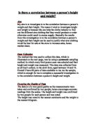
From the results on the table I plotted another scatter graph to show the correlation between height and weight in females. This scatter graph shows a more precise representation of heights and weights, as it is gender specific. The reason for this is that females are generally shorter and lighter than males. This will be shown later.
To create the 30 random male samples I will use the same stratified sampling technique. The formula this time needs to discount the females so the formula I will now use is: number of boys in year x number of samples
Total number of boys in school
Again I will draw a table to show the pupils whose numbers were picked by the calculator.
From the pupils results I can plot a scatter graph, I expect the boys’ height to be greater than the girls’ is so the graph should show a steeper line of best fit. This is a comparison that could not be shown on the first scatter graph due it not being gender specific.
I will now work out the gradient for each graphs line of best fit.
To work out the line of best fit on the graph showing the whole school I will use the formula; y = m x + c
The 2 points I have chosen on the line are (0,12) and (170,56)
M= the y increase
the x increase
= 44
170
= 0.2588..
C= y intercept
= 12
Check Y=0.26 x 170 + 12
= 56.2
The gradient of the line is y=0.26x +12
The gradient of the line of best fit on the scatter graph showing correlation between height and weight in males is:
The 2 points I have chosen on the line are (0,5) and (170,61)
M= the y increase
the x increase
= 56
170
= 0.329..
C= y intercept
= 5
Check y=0.33 x 170 + 5
= 61.1
The gradient of this line is y=0.33x +5
The last gradient to find is from the female scatter graph.
The 2 points I have selected from the line are (0,12) and (175,60)
M= the y increase
the x increase
= 48
175
= 0.2742…
C= y intercept
= 12
Check y=0.27 x 175 +12
= 59.25
The gradient of this line is y=0.27x +12
Comparing the male line of best fit with the female line, I noticed that the gradient of the males is steeper than that of the females, this matches my initial prediction and shows that males are taller and heavier than females.
I worked out the mean, overall total divided by how many points were added together. For the males this was the point (162.4,55) and for the females (157.5,48.9). I noticed that the mean, which I plotted on my graphs, was higher in males, also proving that males are heavier and taller than females.
By drawing a cumulative frequency curve I can compare the medians and also draw a box plot using the results of the curve, this will also help show the differences between height and weight in females and males.
I will use the same 30 samples of males and females as I have used to plot the scatter graphs, I have already drawn up frequency tables under each table of gender sampling.
By drawing the curves on the same graph it is easier to compare the 2 different curves and medians.
From the cumulative frequency I can find the lower quartile, median and upper quartile.
The lower quartile is found exactly 1 quarter of the way up the y axis (cumulative frequency) by drawing a straight line from that point to the line and then from the line down the vertical axis. This point on the x-axis is the lower quartile.
The median is found by doing the same, except that the line is taken from exactly half way up the cumulative frequency axis. The point that the line meets on the x-axis is the median.
The upper quartile is found exactly 3 quarters of the way up the cumulative frequency axis and the point that meets the axis is the upper quartile.
These points are labelled on my cumulative frequency graph as follows:
Lower Frequency Q1
Median Q2
Upper quartile Q3
By taking the quartiles and median that I found from my cumulative frequency curve I could plot a box and whisker diagram. From this you can clearly see that the both the lower and upper quartile, and the median on the males diagram is higher than that of the females showing that males are taller on average. The range of the females is larger than the boys although both upper ends of the range are 180cm. This shows that some girls are as tall as boys are, but this may be due to results being to the extremes as the quartile range is lower than the boys.
From this investigation I have concluded that there is a positive correlation between height and weight, in both males and females. By developing my results and plotting scatter graphs and working out the gradient of the line of best fit I could show that boys were generally heavier and taller than girls. This matched my initial predictions and was confirmed when I plotted a cumulative frequency curve and box and whisker diagram. The box and whisker plot showed the medians and ranges, which helped compare the genders more effectively. This confirmed that males were generally taller and heavier than females.