2 Discuss the strengths and weaknesses of each of the following techniques used to estimate the ERP
- a. Historical Data Approach
- b. Gordon Growth Model Approach
- c. Price Earnings Ratio Approach
The Equity Risk Premium (ERP) can be estimated via 3 methods, namely thru’ the use of Historical Data, the Gordon Growth Model or thru’ the Price-Earnings Ratio approach. The respective strengths and weaknesses of each of these approaches are discussed in the following sections:
a. Historical Data Approach. The Historical Data Approach towards estimating ERP utilizes differences over annual returns in stocks and bonds over a long time period to estimate forward ERPs. A considerable time period is required to provide some level of credibility to estimated forward ERP. In the US, historical data can go as far back as the 1800s. One of the key strengths of using historical data to estimate ERP is the ease of obtaining the estimate, i.e. by studying trends related to the mean returns in the past to project future values of ERP. There are several criticisms, though, of using this approach, chief of which is the length of the time period used to calculate ERP. Longer time periods invariably result in lower standard errors. This problem is especially evident in emerging markets, where there is a shorter time period from which to obtain the data. Furthermore, the period chosen may not accurately reflect the outcome in the future (e.g. certain events are one-off incidents in history). Another weakness lies in the choice of using either arithmetic average or geometric average to estimate the returns on stocks, bonds and bills. An arithmetic average would be ideal to provide an unbiased estimate of the ERP for the next year if annual returns are uncorrelated over time. However, the geometric average seems to be a better choice if returns on stocks are negatively correlated over time. One other criticism of this approach lies in the choice of treasury bills or bonds as the risk free rate. Any premium earned by stocks should be over this chosen rate and thus it is advisable that the risk free rate chosen has to match up to the duration of the cash flows being discounted. Lastly, the underlying assumption used in the historical data approach is that investors’ risk premium have not changed over time and the average risk investment in the market portfolio has remained stable over the period examined. This is highly debatable and the assumption may not hold.
b. Gordon Growth Model Approach. As compared to the historical approach for calculating ERP, the Gordon Growth Model (GGM) is forward looking in that it assumes a constant dividend growth rate in the future. The Gordon Growth model is a simple and common version of the Dividend Discount Model (DDM). This approach is a reasonable approximation for many developed country economies. One idea is to estimate growth in real dividends and real earnings based on GDP; however, this is highly debatable as earnings growth may not be as fast as GDP. Thus, a key strength of using the GGM is that it’s useful for valuing stable-growth, dividend paying companies as well as stock indices (as in the Case discussion). One key weakness of the GGM to estimate ERP is that it is too simplistic to assume that dividend growth would be in line with GDP growth. For most companies, this may be an overestimate, and hence the ERP calculation may be biased upwards. Furthermore, new technological advances may be available in the future which may lead to higher growth rates which may apply to selected sectors of the economy. Perhaps a 3-stage DDM may provide a better approximation.
c. Price Earnings Ratio Approach. The Price Earnings Ratio approach to estimate ERP utilizes the Earnings Yield (i.e. E/P, which is the inverse of the P/E ratio). The earnings yield would measure a company’s real return as retained earnings are re-invested at its quoted P/E ratio. A key strength with this approach lies in its simplicity to calculate the ERP. One key assumption though is that returns in any form of investment by the firm are similar. A weakness with this approach lies in the fact that it may be too simplistic to assume returns from any form of investment by the firm would be similar. Another weakness lies in the fact that the earnings yield is based on past data and it is assumed that these values are going to hold in the future.
-
What would your estimate of the US Equity Risk Premium for the following 1 year be? You can use any or all 3 of these approaches. You should use current data from whatever sources you can obtain to derive your ERP.
Historical Data Approach. The first method to calculate ERP is to use the Historical Data approach, which remains the standard approach when it comes to estimating risk premiums. The actual returns earned on stocks over a long time period is estimated, and compared to the actual returns earned on a default-free (usually government security). The difference, on an annual basis, between the two returns is computed and represents the historical equity risk premium. While users of risk and return models may have developed a consensus that historical premium is, in fact, the best estimate of the risk premium looking forward, there are surprisingly large differences in the actual premiums observe being used in practice. There are three reasons for the divergence in risk premiums:
a. Time Period Used. While some use data dated back to 1927, others use shorter period of time, such as fifty, twenty or even ten years to determine historical risk premiums. The rationale for using shorter periods is the change of average investor’s risk aversion over time, and hence provides a more updated estimate. However, this has to be offset against a cost associated with using shorter time periods, which is the greater noise in the risk premium estimate. In fact, given the annual standard deviation in stock prices returns between 1927 and 2007 is 20%, the standard error associated with the risk premium estimate is estimated for different periods:
To get reasonable standard errors, long time periods of historical returns are needed. Conversely, the standard errors from ten-year and twenty-year estimates are likely to almost as large as or larger than the actual risk premium estimated. This cost of using shorter time periods seems to overwhelm any advantages associated with getting a more updated premium.
b. Choice of Risk free Security. The Ibbotson database reports returns on both treasury bills and treasury bonds, and the risk premium for stocks can be estimated relative to each. Given that the yield curve in the United States has been upward sloping for most of the last seven decades, the risk premium is larger when estimated relative to shorter term government securities (such as treasury bills). The risk free rate chosen in computing the premium has to be consistent with the risk free rate used to compute expected returns. Thus, if the Treasury bill rate is used as the risk free rate, the premium has to be the premium earned by stocks over that rate. If the Treasury bond rate is used as the risk free rate, the premium has to be estimated relative to that rate. For the most part, in corporate finance and valuation, the risk free rate will be a long term default-free (government) bond rate and not a Treasury bill rate. Thus, the risk premium used should be the premium earned by stocks over treasury bonds.
c. Arithmetic and Geometric Averages. The final sticking point when it comes to estimating historical premiums relates to how the average returns on stocks, treasury bonds and bills are computed. The arithmetic average return measures the simple mean of the series of annual returns, whereas the geometric average looks at the compounded return. Conventional wisdom argues for the use of the arithmetic average. If annual returns are uncorrelated over time, and the objective is to estimate the risk premium for the next year, the arithmetic average is the best unbiased estimate of the premium. In reality, there are strong arguments for the use of geometric averages. First, empirical studies indicate that returns on stocks are negatively correlated over time. Consequently, the arithmetic average return is likely to overstate the premium. Second, while asset pricing models may be single period models, the use of these models to get expected returns over long periods (such as five or ten years) suggests that the single period may be much longer than a year. In this context, the argument for geometric average premiums becomes even stronger.
In summary, the risk premium estimates vary across users because of differences in time periods used, the choice of treasury bills or bonds as the risk free rate and the use of arithmetic as opposed to geometric averages. The effect of these choices is summarized in the table below, which uses returns from 1927 to 2007.
Note that the equity risk premiums range from 3.2& to 7.8%, depending upon the choices made. In fact, these differences are exacerbated by the fact that many risk premiums that are in use today were estimated using historical data three, four or even ten years ago.
To conclude, this paper based on historical data approach to forecast 2009 Equity Price Premium (ERP) based on: (1) Stock less Treasury Bonds (2) Geometric Mean method and (3) a long duration period of 80 years (1927-2007). As such, this paper calculated the expected ERP in the region of 4.62%.
Gordon Growth Model Approach. For equity return estimation, forward S&P500 return are calculated.
By re-arrange the GGM: P = D / (K-g)
Equity return can be estimated as K = D / P + g
Where P: S&P 500 index, D: S&P 500 index Dividend and D/P is dividend yield of S&P 500 index, g: Real GDP Growth
D/P is estimated to be 2.24% in the following one year (source ) and real GDP growth is estimated to be 2.9% (source: ).
Hence estimated equity return K = 2.24% + 2.9% = 5.14%
For risk free security estimation, 10 year Treasury Inflation Protected Security (TIPS) are used to calculate the risk free rate. Because the coupon payments and principal are adjusted semi-annually for inflation, the TIPS yield is already a real yield. TIPS are not truly risk-free; if interest rates move up or down, their price moves, respectively, down or up. However, if we hold to maturity, the real rate of return can be locked.
TIPS Real Yield = 1.69% according to latest data Aug 22, 2008
ERP = K- TIPS Yield = 3.45%
Earning-based Approach. To estimate equity return, forward P/E ratio is used as:
K= 1 / (P/E) where P/E is forward Price to earnings ratio estimation of S&P 500 index
Forward P/E for S&P are estimated to be 16.76 (source )
Hence real equity return K = 1 /16.76 = 5.96%
For risk free security estimation, 10 year Treasury Inflation Protected Security (TIPS) are still used to calculate the risk free rate.
TIPS Real Yield = 1.69%
ERP = K- TIPS Yield = 4.27 %
As a summary, all three approaches give similar results as follows:
Further analysis suggests GGM approach gives the most reliable result because it takes into consideration both the future dividends as well as future growth. In contrast, an earnings-based approach does not consider the future growth. Historical approach may give an accurate result if a relatively long time period is utilized in the analysis. However, the result may deviate significantly from the actual value in a fluctuating & emerging market.
REFERENCES:
-
“Estimating Equity Risk Premiums”, Aswath Damodaran, NYU Stern School of Business, accessed (27 Aug) on http://www.stern.nyu.edu/fin/workpapers/papers99/wpa99021.pdf
- For the historical data on stock returns, bond returns and bill returns check under "updated data", accessed (27 Aug) on http://www.stern.nyu.edu/~adamodar