I am going to approach this investigation first by reducing the amount of data I have, as the amount of data is too large to work with comfortably. I am going to do this by using stratified sampling to select 10% of boys and 10% of girls from year’s seven to eleven. I am going to use stratified sampling so that my data is proportional to the number of pupils in each year and my investigation will be fairer and also helps me to reduce the number of data samples I need to use without being biased.
Using this data I am going to create frequency tables but the data will not be split into age groups, as my investigation will be on the students in general, regardless of what year group they are in. I will create two frequency tables, one for the boys in Mayfield High School and one for the girls.
From these tables I will be able to find the median height for the boys and then for the girls. I will do this so that I can compare these figures to the ones that I will obtain later from my graphs. Also from these tables I will find the standard deviation. I will do this to certify that I have a fair spread of data from my stratified sampling for the girls and the boys to ensure a fairer test.
Again using these tables I will go on to produce 2 histograms. One representing the data of the heights of the girls at Mayfield High School and one representing the boys. These histograms will give me a fair idea of the pattern my data has produced but will not be enough to draw a conclusion from.
Therefore on my histograms I will add a frequency polygon to try and see the shape of the histogram from a more accurate view and also to help me produce a girls and boys distribution curve to further help produce an answer to my investigation.
After this, I will find the upper quartile, lower quartile, median and inter quartile range by drawing and box and whisker diagram. I will find the median so that I can compare these figures with the ones I established earlier from the frequency table. I will find the upper quartile, lower quartile and again use the median I will then use my frequency tables to produce a stem and leaf diagram so which will allow me to make a direct comparison between the two sets of data (the boy’s data and the girl’s data).
Then I will produce a stem and leaf diagram, which will allow me to make a more direct comparison between the two, sets of data. I will produce these by using the data I have collected on my spreadsheet
Using these different tables, graphs, and diagrams I hope to produce a good conclusion to the investigation of the hypotheses.
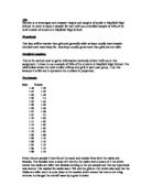
I collected my data and this is how it looks like. I have converted the data into centimetres so that I could use a steam and leaf diagram, as it does not go into 2 decimal places. Using this data I have found the overall mean and median to see whether my hypothesis was correct that boys are taller than girls. The mean for the boys was 165 centimetres while the girls were 160 centimetres. This means that the boys are taller than the girls. The median for the boys is 167 while the girls were 152.5, which means that the boy’s median is bigger and they are taller.
Box and Whisker Diagram
We can tell first of all from the Box and Whisker Graph, on the page above, for height that the boys have an interquartile range that is larger then the females showing that the females are more compact and are closer together, and are more even in height then the males. Also the upper quartile is larger for males but the lower quartile is smaller than the females showing that the male’s data is more disperse in the middle 50% and that males have taller males than females but also have shorter. The middle 50% is a good measure of spread as it shows the normal and not the extremes. Using this data to my hypothesis I would have to say that the females are more constant in height and that in the males they may have quite a few extremes but the medians are the same so if you were to take everyone on average then neither would be taller. Also from the box and whisker diagram we can see that the girls are quite negatively skewed while the boys are slightly positively skewed which tells us that there are taller people in that sample for the boys as they are positively skewed and less tall people for girls as they are negatively skewed. This supports my hypothesis as there is more boys who are taller than taller girls.
Female
Male
Histogram
From my histogram on the other page we can tell that most of the people are all in the middle few bars but in the last bar there are more boys than girls. The frequency density in the class range 165<h<190 for boys are 1.08 while the girls are 0.72 which shows that there are more taller boys than girls and the shortest class range for boys and girls were both 2.7. Although from this we can say that there are more taller boys than girls it does not completely justify my hypothesis as in the class boundary 160<h<165, which is the 2nd largest class boundary, the girls have a larger frequency density than boys as the girls had 3.2 while the boys had 2.2. This does not support my hypothesis and therefore we cannot say which is taller but we can say that there are taller boys than girls.
Standard Deviation
The standard deviation shows the average variation from the mean line, for whole range of data. For example, if the standard deviation were 0.23, that would mean the total average of all the data points would be 0.23 points away from the mean data line. I used the function on the excel database to calculate the standard deviation, both to save time and to ensure that I got the calculations right.
The male’s Standard Deviation was 13.483cm and the female’s were 10.652cm.
From this I can say that this does not support my hypothesis, as the male’s data is more disperse and the female’s choice of data was better as it was closer together.
Evaluation
There are many things I could have done to improve my data and my investigation. I could have improved my data and its sample by using a bigger sample and getting a more reliable result for the whole school by chosen more people and having a bigger sample. Also the data was second hand and all the data may have been slightly incorrect or wrong.
Conclusion
Using the data I have found from this investigation I can now say that on average boys are taller than girls as the males had 1.705 and the girls is 1.61 but the boys also had a bigger range. This supports my hypothesis and my hypothesis was correct as boys were taller than girls but also there were many short boys and their data was very disperse as we found in the box and whisker diagram and in the standard deviation. Also from the histograms we saw that there were taller boys than girls but there were also shorter boys. As my overall findings are that boys on average were taller than girls I can not make this judgment about the whole school as I took too small of a comparatively small sample, and the data represented from this investigating is not enough evidence to back-up my findings definitely.