∑f 49
Girls’ Height
Mean = ∑fx = 7925 = 161.7 cm Modal Class Interval = 160 ≤ w < 170
∑f 49
Boys’ Weight
Mean = ∑fx = 2220 = 55 kg Modal Class Interval = 50 ≤ w < 60
∑f 51
Boys’ Height
Mean = ∑fx = 8345 = 163.6 cm Modal Class Interval = 160 ≤ w < 170
∑f 51
Girls’ Weight Boys’ Weight
Conclusion
All three measures in the sample were higher for boys than for girls; however the sample for boys was much more spread out than the girls, where the range in the sample for boys was 66kg and the range in the sample for girls was 36kg. This is supported by the frequency polygons and the histograms, on the previous pages, as they show that the lightest and heaviest weight comes from the boys’ part of the sample, meaning that the boys must have a higher range than the girls.
The evidence that has been gathered from the sample implies that 14 out of 51, or 27% of the boys have a weight between 50 and 60 kg, whereas 21 out of 49, or 43% of the girls have a weight between 40 and 50kg. The frequency polygons show that there are no girls over the weight of 70kg, but 16% of boys are. Although there are a small number of boys with a lighter weight than some girls and a small number of girls with a heavier weight than some boys, the evidence suggests that in general, the weight for boys is greater than the weight for girls.
Girls’ Height
Conclusion
In the sample, the mean and median height was a little higher for the boys than for the girls, but the modal height was the same for both with a class interval of 160-170 cm. The sample for boys was more stretched, with a range of 70 cm compared to 60 cm for the girls. The evidence from the sample suggests that 18 out of 51, or 35% of boys have a height between 160 and 170 cm, whilst 19 out of 49, or 39% of girls have a height within the same boundaries. The evidence shown in the table above suggests that the distribution of height between girls and boys is fairly similar. However, the frequency polygons and the histograms drawn for the boys and girls illustrate that there are more girls that have a height below 170 cm than boys, but more boys have a height above 170 cm than girls. Even though there are more girls than boys in the overall modal class interval, the sample demonstrates that in general, the height for boys is greater than the height for girls. This means that my prediction was correct in saying that boys are likely to be taller and heavier than girls.
Evaluation
I used many techniques in my pre-test. I used the frequency tables efficiently where I was able to find the mean from grouped data. After I had created the frequency tables, I produced four stem and leaf diagrams, comparing the girls and boys, so that I could easily work out the median and gain an accurate analysis of the specific weights and heights of the girls and boys. Once this was done I was able to create the histograms. I am investigating two pieces of continuous data (height and weight) so histograms would be an appropriate piece of presentation to illustrate the different heights and weights in my sample. I did not use any pie charts as they would be inappropriate to represent the data and would make difficult to read and interpret the results.
The conclusions that have been found on the relationship between height and weight are based on a stratified sample of 51 boys and 49 girls, which eliminated the factor of bias and the growing number of students in Mayfield High School. To confirm the results that were found, I could extend the sample or repeat the whole investigation with a different sample and compare the two sets of results.
I think that my conclusions are quite reliable as they comment on the relationship between height and weight considering gender and suggest that there is a relationship, which will be looked at further on in the investigation. However, I think that the range that was found is quite unreliable to use in the conclusion. This is because the two extreme values created a big range, especially for the boys, meaning that the results would be affected, and could be proved to be unreliable. To improve this, I would find out the interquartile range as it does not take the highest and lowest values, but the upper and lower quartile, meaning my conclusion could be strengthened.
Overall my strategy worked quite well. This is because I gained accurate results by making it a fair sample through the use stratified sampling. The bias of age and gender that would have affected my results was eliminated due to my stratified sample, which I randomly sampled after. The histograms and frequency polygons that I used effectively allowed me to compare the heights and weights of girls and boys and see the trends within the relationship between height and weight, which included the formation of a new hypothesis, which is:
‘In general, the taller a person the heavier that person is likely to be’.
This means that my prediction in saying that the taller a person the heavier is correct, which also implies that there is a strong relationship between height and weight. The new hypothesis that has been formed will be looked at in detail in the next section of the investigation.
I think that the idea of the creation the histograms and frequency polygons for girls and boys alongside each other was beneficial as they allowed me to easily see any trends and patterns that should be included in my conclusions. This was a vital part of my strategy to enable me to compare the data efficiently.
Extension
Hypothesis
- In general, the taller the person is, the heavier that person is likely to be.
Plan
I have now found a new hypothesis to study. I am going to try and show that in general, the taller the person is, the heavier that person is likely to be. To investigate this hypothesis I will need a new random sample of 50 students of any gender. It will be random because I need to make sure that every student has an equal chance of being selected to be in my sample. I do not need to use stratified sampling as I am not investigating boys and girls. I am only trying to prove that if a person who is randomly selected is tall, the heavier they are likely to be. The data that is randomly sampled will be used to do this. After I have sampled the data, I will have a table that only consists of the heights and weights of 50 randomly selected students.
To compare this sampled data, I will produce a scatter diagram of height against weight. This will enable me to see any trends that will appear, or, in other words, if there is any correlation between height and weight. The scatter diagram is a good way to compare the points that are plotted as height against weight as a general trend can be seen straight away.
If there is a positive correlation, then the hypothesis that is being tested will be true. This means that there is a direct correlation between height and weight, where the greater the height means the greater the weight. If there is a negative correlation the hypothesis will be answered as false. This is very unlikely to happen, however there may be a few exceptions that may occur, which do not follow the general trend. To spot these exceptions as well as spotting the trend, I will draw a line of best fit. This will show me the trend straight away when I look at the scatter diagram and so I will be able to interpret it easily when I am constructing a conclusion. The line of best fit will also enable me to predict a weight from a given height. I can compare the data like this as well by taking one large height and one small height and comparing the weights that are given from the line of best fit.
Limitations
Similar to the first section of the investigation, there are limitations that involve the different lifestyles of students that cannot be controlled. This means that there are diverse diets and also different metabolic rates that could affect the height and weight of each student. This then implies that there are bound to be exceptions to the general trend within the scatter diagram.
Conclusion
You can see on the scatter diagram that there is a positive correlation between height and weight. This means that the larger a person’s height, the heavier that person is likely to be. The line of best fit suggests that a person with a height of 155 cm will be 47 kg, whereas a person of a height of 175 cm will be 56 kg. This shows the difference that height of a person makes towards the weight of that same person. This is that the greater the height, the greater the weight is likely to be. This statement answers my hypothesis as true.
The scatter diagram helped me show that the hypothesis was correct. It was the fact that it caused a general trend to appear when height was plotted against weight. A line of best fit made this clearer as it presented the trend so that it could be seen more easily effectively. However there are a few exceptions that can be seen on the scatter diagram that are opposed to the general trend. For example the person with a height of 152 cm has a weight of 70 kg, but the person who has a height of 180 cm has a weight of 57 kg. According to my line of best fit, the person with a height of 153 cm should have a smaller weight than the person who has a height of 180 cm, but reality disagrees with that theory. These exceptions occur because of the different diets of the students and the dissimilar metabolic rates that each one has. These are factors which cannot be controlled by a researcher so there are likely to be exceptions. Therefore, my first hypothesis is a fair statement to use when commenting on these results as it uses the factor of probability in its wording:
‘In general, the taller a person is, the heavier that person is likely to be’.
Evaluation
The random sampling that I used made this part of the investigation fair. Every student was equally likely to be selected so I got firm results that were not biased. To improve the results I got and strengthen them, I could extend the random sample, or even repeat this experiment with a completely different random sample of 50.
My conclusion is reliable as the results clearly show that there is a positive correlation between height and weight. However, the plotted points are a little spread out, which makes it a little bit difficult to spot a clear trend. Although the line of best fit fixes this, the overall conclusion could be argued as unreliable. This means that there should be another way that the correlation can be made even better in a scatter diagram. This is where the factor of gender should be considered. The sample could have been slightly biased if more girls were randomly selected than boys, or if it was the other way round. This is because in the scatter diagram, it could be difficult to find a line of best fit because of all the different heights and weights that are affected by gender. However, the purpose of this part of the investigation was to explore the hypothesis of:
‘In general, the taller a person is, the heavier that person is likely to be’.
This was answered as true and so we now know that there is this correlation between height and weight. This can lead on to another extension to the line of enquiry, where a new hypothesis should be tested that involves gender. This is that:
‘There will be a better correlation between height and weight if boys and girls are considered separately’.
Further Investigation
Hypothesis
- There will be a better correlation between height and weight if boys and girls are considered separately.
Plan
In the early section of this investigation, or, in other words the pre-test, evidence was found that suggested that height and weight were both affected by gender. I am now trying to show that there is a better correlation between height and weight if girls and boys are considered separately.
To investigate this hypothesis, I will need to use the stratified sample that I created before of 51 boys and 49 girls so that the data that I interpret will reflect the whole population of Mayfield High School. The use of stratified sampling will also eliminate the bias of age that may occur in this part of the investigation. This means that I will have accurate results within my sample.
At first, the sample that I use will be presented in three scatter diagrams (one for boys, girls and the mixed population in the sample). These diagrams will have a scale from 20 to 100 on the y-axis, and 120 to 200 on the x axis. This will allow me to compare the different results and see if the correlation has become stronger after a line of best fit is drawn. After this, I will find the equations of the lines and use them to make predictions and analyse the data further by predicting different weights when the height is known and heights when the weight is known. I will need to find the y-intercept first as I do not have an origin. This will be done by making c the subject of the formula y = mx + c.
As I am dealing with two pieces of continuous data, height and weight, cumulative frequency diagrams would be appropriate and a powerful tool to compare the different data sets. I will need to create a cumulative frequency table for height and weight separately and then draw cumulative frequency curves for boys, girls and the mixed population in my sample on the same graph. On my cumulative frequency graphs, I will only demonstrate how to find the median and interquartile range for the mixed population so the graphs will still stay clear. Through these diagrams, I will be able to find the median and the interquartile range. This will allow me to draw box-and-whisker diagrams, which will allow me to make further comparisons between girls and boys. I will also predict percentages of students who have a height or weight within a given range. This will consider ranges other than the interquartile range, which ignores 50% of the students. I can analyse distinct ranges when dealing with percentiles. The cumulative frequency graphs will also allow me to see the relationships between the data for boys and the data for girls, which I can conclude from.
There is a positive correlation between height and weight when girls are considered.
There is a positive correlation between height and weight when boys are considered.
Conclusion
The evidence gained from the scatter diagrams supports the hypothesis. This is that there is a better correlation between height and weight if girls and boys are considered separately. The correlations for girls, boys and the mixed population were all positive. They have all became better from the previous scatter diagram for the hypothesis of, ‘In general, the taller a person is the heavier that person is likely to be’. The diagrams made for the girls and boys had a much better correlation to the combined sample, which did not have as good a correlation as the diagrams for height and weight when girls and boys were considered separately. This means that there can be better results found for the relationship between height and weight if boys and girls are considered separately. The lines of best fit were drawn with ease, because of the better correlations that was formed.
As the correlations for the girls and boys were quite different and now it is known that there is a better correlation when boys and girls are considered separately, the hypothesis made in the first section of this investigation, which was, ‘the relationship between height and weight is affected by gender’, can further be proven as true. This is presented on my scatter diagrams through the lines of best fit. For example, the lines of best fit on my diagrams predict that a girl who is 160 cm tall would have a weight of 49 kg, whereas a boy of the same height would have a weight of 53 kg. This comparison shows that boys are likely to be heavier than girls even if both genders are of the same height.
The lines of best fit that I have created are straight lines. This means that you can find the equations of these lines by using the formula, ‘y = mx + c’ by finding the gradient of the line and the y-intercept. The y-intercept will need to be worked out as I do not have a graph with two quadrants or an origin. This is done by working out the gradient, putting in any values for x and y and then making c the subject of the formula in y = mx + c. Here are the y-intercepts for the data set:
Boys: c = y – mx = 40 – 87.5 = - 47.5
Girls: c = y – mx = 40 – 58.5 = - 18.5
Combined Sample: c = y - mx = 40 – 80.62 = - 40.6
If y represents weight, and x represents height, the equations of the lines of best fit for the data set are:
Boys: y = 0.625x – 47.5
Girls: y = 0.45x – 18.5
Combined Sample: y = 0.556x – 40.6
Now that I have these equations, the weight can be predicted when the height is known, or height when the weight is known. For example to predict the weight of a boy who is 170 cm tall:
y = 0.625x – 47.5 x = 170
= 106.25 – 47.5
= 58.75 kg
Since weight is a continuous piece of data, it can be appropriate to have a value with a decimal point. In fact, the use of the decimal point makes the value more accurate, meaning that my predictions will be more accurate.
Evaluation
The conclusion that I gained from the scatter graphs was reliable. It commented on the general trend and proved that there is a better correlation between height and weight when boys and girls are considered separately. But there were a few exceptional values that fell out of the trend. For example in the scatter graph for boys, there is a boy who has a height of 162 cm, but has a weight of 92 kg. According to the line of best fit, the boy should have a weight of about 49 kg. This has probably happened because the boy has a different diet to the average student, or it could be that he has a different metabolic rate. These factors are ones that cannot be controlled and so it is likely that there are some values, which fall out of the general trend.
Cumulative Frequency for Weight
Cumulative Frequency for Height
Conclusion
Here are the findings from the cumulative frequency curves for weight:
This can be represented on a box-and-whisker diagram shown below:
The box-and-whisker diagrams for weight show that the girls’ interquartile range was 8 kg less than the boys. This suggests that the boys’ weights were more spread out than the girls. However, the interquartile range for the mixed population was less than the interquartile range for the boys. This implies that the boys’ weights were slightly more spread out than the whole population in the sample. This is probably because the girls, who have less spread out weights than boys, had a bigger impact on the whole sample than the boys did and so the sample was made to be less spread out due to the values corresponding to the girls that were also less spread out.
Here are the findings from the cumulative frequency curves for height:
This can be represented as box-and-whisker diagrams shown below:
The box-and-whisker diagrams show that the girls’ interquartile range was 7 cm less than the boys’. This suggests that the boys’ heights were more spread out than the girls’. The interquartile range for the boys’ was 1 cm more than the interquartile range for the mixed population. This implies that the boys’ heights are more spread out than the mixed population.
I also used the cumulative frequency curves for height and weight to predict percentages of students that had a height within a given range. For example I estimated how many boys in my sample had a weight between 50 and 65 kg. I done this by reading off my cumulative frequency curve for boys’ weight to see how many boys had a weight up to 50 kg. This was 20 boys. I then read how many boys had a weight up to 65 kg; this was 39 boys. This meant that 39 – 20 = 19 boys had a weight between 50 and 65 kg. Since my sample is proportionate to Mayfield High School, I can use that figure to estimate that 19/51, or 37% of boys in the school will be between 50 and 65 kg heavy. This suggests that if a boy is selected at random from the school, the probability of him having a weight between 50 and 65 kg is 0.37.
The same estimation can be made for heights, but first I can find out the heights for boys that will be found from a weight of 50 kg and 65 kg when the equations of the line of best fit is used, which I found previously on the scatter graph for boys:
y = mx + c y = 50, m = 0.625, c = - 47.5
x = 50 + 47.5 = 156 cm
0.625
y = 65, m = 0.625, c = - 47.5
x = 65 + 47.5 = 180 cm
0.625
I can now predict how many boys will have a height between 156 and 180 cm. The cumulative frequency curve for boys’ heights tells me that 13 boys have a height up to 156 cm, and 47 boys have a height up to 180 cm. This means that 47 – 13 = 34 boys in the sample have a height between 156 and 180 cm. Since the sample is a model of the school, I can estimate that 34/51, or 67% of boys in the school have a height between 156 and 180 cm. This means that if a boy is picked at random, the probability of him having a height between 156 and 180 cm is 0.67.
The data suggest that if a boy is picked at random, the probability of him having a weight between 50 and 65 kg would be 0.37. If the boy did have a weight between that range then there would be a probability of 0.67 of him having a height between 156 and 180 cm.
Evaluation
The results that I gained were reliable, meaning that I formed a reliable conclusion. This is because I had many results that I could link together, including the results that I gained from the scatter graphs that I created earlier, where I had concluded with equations of the lines of best fit. I could link a set of data that involved height and weight and proved that there is a strong correlation when boys and girls are considered separately. To improve this part of the investigation, I would probably need to include a bigger sample, or even repeat this section with a new stratified sample.
Summary of the Results
- There is a positive correlation between height and weight. In general, taller people are likely to have a larger weight than smaller people.
- The points on the scatter graph for the girls are less dispersed about the line of best fit than those for the boys. This suggests that the correlation is better for girls than for boys.
- The points on the scatter graph for boys and girls are less dispersed than the points on the scatter graph for the mixed sample of boys and girls. This suggests that there is a better correlation between height and weight when girls and boys are considered separately.
- The scatter graphs can be used to give reasonable estimates of height and weight. This can be shown either by reading from the graph or by equations of lines of best fit.
- The median height and weight for boys is higher than the median height and weight for girls.
- The box and whisker diagrams conclude that, in general, boys are taller and heavier than girls, but not exclusively so. The cumulative frequency curves show that 41% of girls have a weight above 52 kg, the median weight for boys, and 53% of girls have a height above 162 cm, the median height for boys.
Limitations
- My results could have been more reliable if a larger sample had been used, or if some sections of the investigation had been repeated.
- The predictions that I have made are based on general trends that have been observed in the data. In the samples that I had made, there were exceptional values coming from individuals whose results fell outside the general trend. This was because of factors such as the diet, which could not be controlled.
Considering Age
Although I did create a sample in the investigation that was stratified and eliminated the bias of gender and age, I have not studied whether age has a vital role in the height and weight of students. Therefore I am now considering age as one of the main factors that affects the relationship between height and weight.
Hypothesis
- When age is taken into consideration, the correlation between height and weight will be better when age is not considered.
Plan
I am trying to show that there is a better correlation between height and weight when age is taken into consideration. I will need to create a new stratified sample from the whole population in Mayfield High School. I already know that this data is reliable and will enable me to get accurate results. The number of students from each year that I will need in my sample has been constructed in the table below.
I obviously need a stratified sample for this exercise as there are a growing number of students that come into the school each year. This means that there will be more students in Year 7. In order to represent the whole school appropriately, I need to create a stratified sample so that the number of boys and girls from each Year Group in my sample is proportionate to the number of girls and boys in each Year Group in Mayfield High School. This way, I know that by taking a stratified sample, I can be sure that my sample is representative of the whole school. As far as possible, my sample is free from bias caused by gender and age divisions.
Here is a summary of the results for the stratified sample across the year group:
Although these results are sure to represent the whole school, the sample is not yet big enough to make any meaningful statements about the data within each year group. In order to look in each year group in more detail, I will create a 15% sample for each year group and gender. For example, there are 151 boys in Year 7, so a sample of 10% would contain 15.1 boys. Obviously, there cannot be 15.1 boys, so I round the number to the nearest whole number, meaning that the 10% sample of year 7 boys would consist of 15 boys. If there was a number that was exactly in the middle of two numbers, such as 15.5, I would toss a coin to see which number I should use as my 10% sample.
I need to create a 10% sample of year 7 boys. I will make sure that the sample has a frequency table to accompany it and show me the results from the data. This will also help me when I am using standard deviation. Instead of working out the standard deviation for each individual values, I am going to work out the standard deviation for grouped data, where data is given in a frequency table. This means that I am going to use the formula of:
√∑fx2 – x2
∑f
where ∑f = sum of frequency, ∑fx2 = sum of frequency times midpoint2, x2 = mean2
I am going to use standard deviation because it uses all the values of a piece of data and also it is a measure of average dispersion about the mean. The results that I will gain will be very reliable as standard deviation makes use of all the values. The lower the value of standard deviation, the closer most of the data is to the mean and so the results are reliable. This can be put into terms that states that a small standard deviation means that the values do not vary much, whereas a large standard deviation indicates that individual values are more variable. This will tell me whether the results I get are reliable and if age is a vital factor when considering height and weight. To accurately get this comparison, I will work out the standard deviation for the boys in my sample that I created before this.
Year 7 Boys
Boys in the Whole School
Conclusion
The heights of the boys in the sample representing the boys in the whole school appear to be far more spread out than the heights for boys in year 7 alone. The standard deviation for the heights of boys in the whole school was 17.37 cm, whereas the standard deviation for the heights of boys in year 7 was 7.72 cm. This means that the standard deviation for the boys representing the boys in the whole school was twice as much as the standard deviation for the 10% sample of year 7 boys. The relationship between height and weight for the sample of year 7 boys can be represented as a scatter graph below.
Evaluation
You can see that there is a much better correlation between height and weight when age is considered in detail. There are a few anomalies on the scatter graph that fall out of the general trend. This happens as well to the relationship between height and weight with the boys in the sample representing the boys in the whole school. To get better results I could have separately ignored these exceptional results, but chose not to so that I could link my results with reality and try and figure out the factors that cause these values to occur. With the conclusion that I have found, I can say that the hypothesis was correct.
Final Conclusion
The stratified sample of 50 students over age and gender shows that there is a mean height of 157 cm for the boys and 156 cm for the girls, and a mean weight of 50.36 kg for the boys and a mean weight of 47.46 kg for the girls. For both of these results, the range of heights and weights for boys was larger than for the girls. This means that there will be quite a few boys that are under the height of 156 cm (the mean height for girls) and there will be quite a few boys under the weight of 47.46 kg (the mean weight for the girls).
The 10% sample of year 7 boys confirmed that there was a better correlation between height and weight when age was considered in more detail. The standard deviation for the heights of year 7 boys was 7.72 cm, whereas the standard deviation for the heights of the boys in the sample representing the whole school was 17.37. This means that the heights for the boys population in the sample were more spread out about the mean than it was for the heights for year 7 boys. This strongly suggests that there is a much stronger correlation between height and weight when age is considered. Along with this, the earlier part of the investigation suggested that there was a better correlation between height and weight if boys and girls are considered separately. The general comparison that was found between girls and boys was that in general, boys are taller and heavier than girls. If all this is linked together, a final summary sentence can be said:
There is a strong correlation between height and weight if gender and age are considered. Once studied, it is found that in general, boys are taller and heavier than girls.
Throughout this investigation I have found that there is a positive correlation between height and weight both across the school and within each year group. The correlation appears to be much stronger when individual year groups and separate genders are considered. However, I can only support this through the experiment that was done with the year 7 boys compared to the boys in the whole school. If I was to improve my investigation, I would investigate each year group and gender, but this would probably be predictable and I think that I have reliable results from the 10% sample of year 7 boys that can support this conclusion.
I have to remember that the school is only a small population in the world. There are many other factors that affect height and weight such as the lifestyle of people and another possible factor could be the amount of money that a person earns that affects weight. Specifically in the school, there are factors that affect the correlation between height and weight such as the distance away from school and the mode of transport used to get to school. If a person walks to school, he or she is more likely to be lighter in weight than a person who frequently comes to school by car.